UQ in Weather Prediction

UQ in Weather Prediction#

This article is currently under construction.

Introduction#

Weather prediction today is performed via so-called numerical weather prediction (NWP) models. These models are simulation models consisting of a set of partial differential equations describing the physics of the atmosphere [Kalnay, 2003]. There is also a close connection to the numerical models used for climate simulations.

According to [Bjerknes, 1904] the atmosphere can be described by seven basic equations (three momentum equations, thermodynamic energy equation, perfect gas law, conservation of mass, conservation of water). To solve the equations it is required to have suitable initial conditions over the domain of interest, suitable lateral and vertical boundary conditions, and additionally a way of numerically solving the equations.

Starting point is to describe the current state of the atmosphere as accurate as possible. Then the equations are discretized in space and time in order to evolve the current state forward in time and obtain predictions of future atmospheric states.

Weather prediction was traditionally viewed as a deterministic problem. However, the atmosphere is a chaotic system and future atmospheric states cannot be definitively predicted [Lorenz, 1963]. As the output of an NWP model is a single deterministic forecast there is no possibility to assess the uncertainty in this forecast. Therefore, there was a change of paradigm since the early 1990s towards probabilistic weather forecasting. Aim in probabilistic weather forecasting is to obtain a predictive probability distribution rather than only a deterministic point forecast in order to be able to assess and quantify forecast uncertainty directly.

Sources of Uncertainty in the NWP Model#

NWP models suffer from various sources of uncertainties. The two main sources of uncertainty come from the fact that the solutions to the equations strongly depend on the initial conditions and the model formulation, see also uncertainty induced by measurement and by parameterization for a general overview on the respective sources of uncertainty.

As the NWP model consists of a system of partial differential equations, starting values are required to initialize the model. These initial values represent the current state of the atmosphere. Given an estimate of the current atmospheric state the NWP model simulates its evolution for future points in time. The estimate of the current state of the atmosphere is supposed to be as accurate as possible. However, every estimate is subject to errors as it is impossible to to describe the true state of the atmosphere to full extent. Additionally, there are different ways to formulate the model physics and to implement the NWP model. As no model is able to truly describe what happens in the atmosphere but is always only an approximation, the model formulation is subject to errors as well.

Initial conditions for the NWP model are obtained by data assimilation techniques combining (possibly indirect) measurements/observations and the model. Sources of uncertainty come from measurement errors as well as a possibly incomplete network of measurement/observation stations (such as weather stations, buoys, satellites) which is not be able to fully represent all aspects of atmospheric behavior.

With regard to the model formulation uncertainties are introduced by incomplete knowledge of the physical processes in the atmosphere, and therefore inaccurate mathematical representations, parameterizations in the equations or numerical schemes in the implementation.

Methods to Cope with Forecast Uncertainty#

Due to the chaotic nature of the atmosphere, minute errors in for example the initial conditions can grow exponentially during the integration process of the NWP model over time. When running the NWP model only a single time the output is a deterministic point forecast, providing no means of assessing its forecast uncertainty.

Therefore, change of paradigm took place since the early 1990s towards probabilistic weather forecasting [Gneiting, 2008]. In this setting the aim is to obtain a predictive probability distribution for future weather events rather than a single point forecast. Such a predictive distribution explicitly allows uncertainty quantification.

Ensemble Prediction Systems#

Common practice in addressing the uncertainties in an NWP model is the use of so-called ensemble prediction systems (EPS). Instead of running the NWP model only a single time yielding a single point forecast, the model is run multiple times, each time with variations in the parameterizations of the model physics and/or the initial and boundary conditions [Gneiting and Raftery, 2005, Leutbecher and Palmer, 2008]. A forecast ensemble is already a probabilistic forecast taking the form of a discrete probability distribution.

While ensemble systems aim to reflect and quantify sources of uncertainty in the forecast [Palmer, 2002], they tend to be biased and suffer from dispersion errors, typically they are underdispersed [Hamill and Colucci, 1997]. Here, a bias is a systematic forecast error coming from the NWP model. Contrary, dispersion errors reflect a statistical incompatibility of the the (probabilistic) forecast and the observation. To be specific, the variance or dispersion properties of the forecast do not match those of the underlying distribution generating the observation. In case of underdispersion the true observation falls outside the range of the forecast ensemble too often, indicating that the variance of the ensemble is too small with respect to the behavior of the observation.

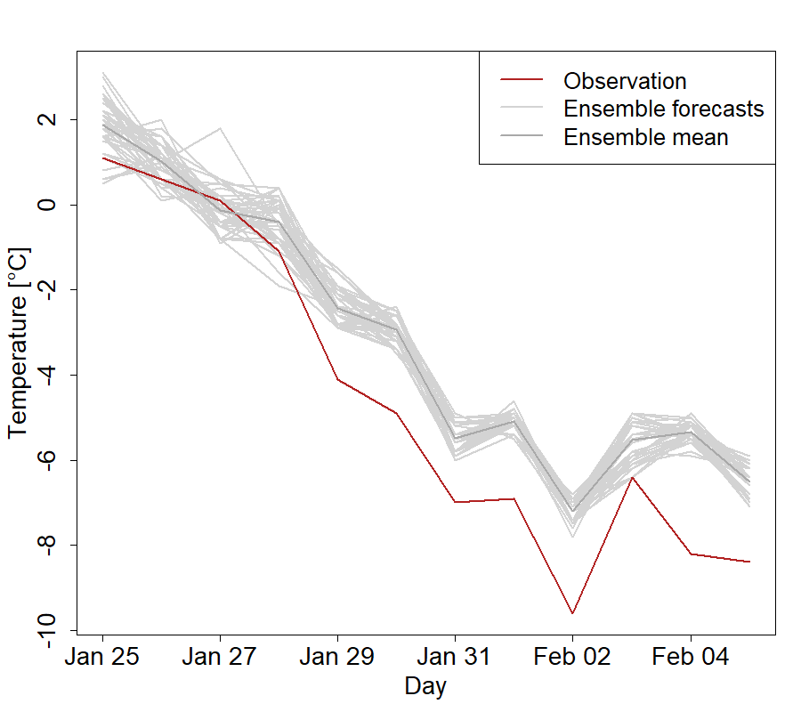
Dispersion error and forecast bias of ensemble forecasts — Fig. 84 Ensemble forecasts for temperature and verifying observation at the station Braunschweig in Germany. The raw ensemble forecasts are often not calibrated with respect to the observation and thus show systematic forecast biases and dispersion errors.#

Fig. 84 shows 50 ensemble forecasts (light grey) for temperature, together with the ensemble mean (solid dark grey) and the acutal temperature observation at the observation station in Braunschweig (Germany) for Janaury and February in 2012.

It is clearly visible that the behaviour of the forecast ensemble is not fully consistent with the observation. Especially after the end of January the observation falls clearly outside the ensemble range, indicating the the range is too small and the dispersion properties need to be adapted. The distance between ensemble forecasts and observation is so large that this also indicates a systematic bias, in this case the ensemble forecasts are systematically predicting a too high temperature compared to the truth. Furthermore, at the beginning of February, the ensemble forecasts predict an increase in the temperature level while the actual observation drops, this also indicates a systematic bias in the forecasts.

Statistical Postprocessing of Ensemble Forecasts#

The calibration and forecast skill of an ensemble forecast can substantially be improved by performing so-called statistical postprocessing to the model output. A postprocessing model corrects the forecasts in coherence with recently observed forecast errors [Wilks and Hamill, 2007]. Typically, statistical postprocessing techniques are probabilistic in nature and return full predictive distributions, see e.g. [Gneiting and Raftery, 2005] or [Gneiting and Katzfuss, 2014].

There are two state-of-the art statistical postprocessing models which form the basis for modifications and extensions in current research, namely

Ensemble model output statistics (EMOS)
Bayesian model averaging (BMA)

The EMOS approach fits a single parametric distribution using summary statistics from the ensemble, e.g. based on a multiple (linear) regression framework [Gneiting et al., 2005].

In the BMA approach each ensemble member is associated with a member specific kernel density function and a weight reflecting the member’s skill. The BMA predictive density is then given as a mixture density of the individual densities [Raftery et al., 2005].

Depending on the weather quantity that is postprocessed an appropriate assumption has to be made with regard to the predictive distribution. Popular choices are for example

Normal distribution for temperature and pressure
Gamma, log-normal or truncated normal distributions for wind speed
Generalized extreme value distribution left-censored at 0, left-censored and shifted gamma distribution or a discrete-continuous mixture for precipitation
Multinomial distribution for cloud cover.

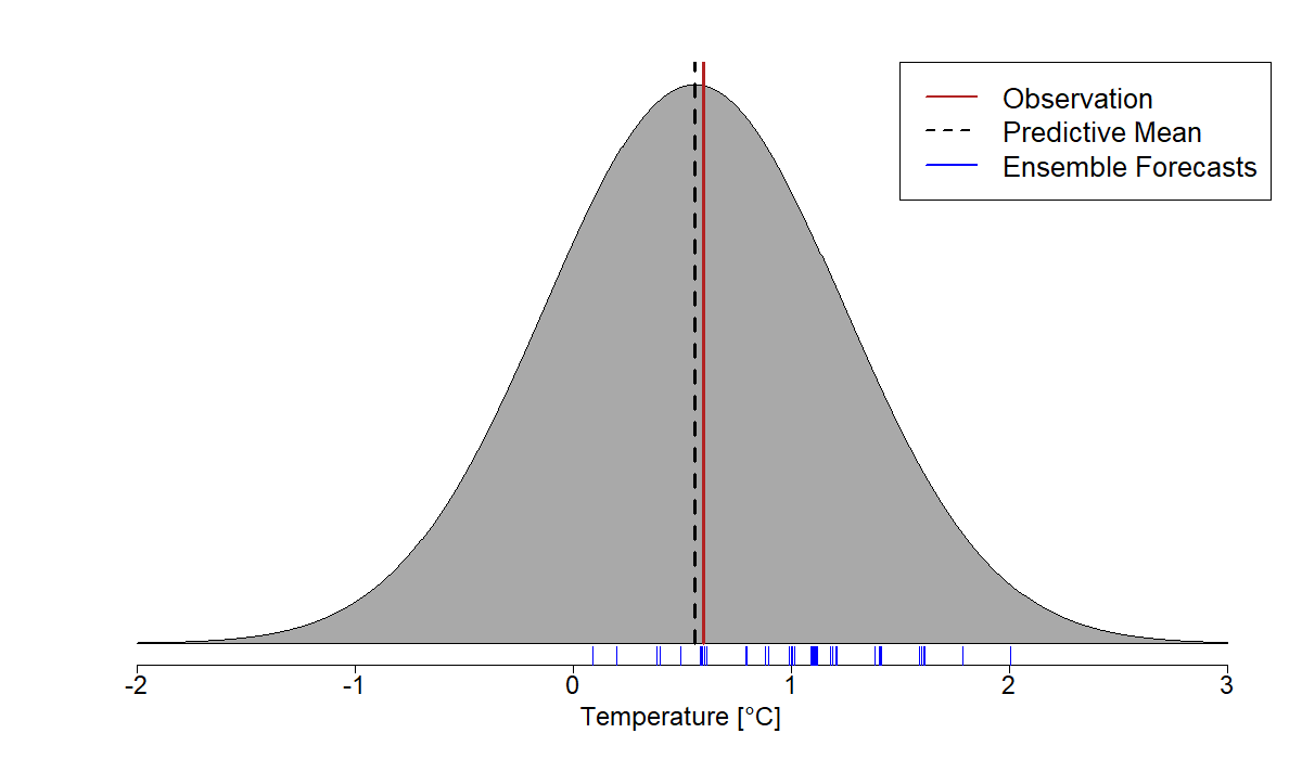
Predictive distribution for temperature obtained by the EMOS model — Fig. 85 A predictive normal distribution obtained by the EMOS model. While the raw ensemble forecasts (blue) are not calibrated with respect to the observation (red), the postprocessed probabilistic forecast is centered with respect to the observation and its predictive mean (dashed black) is close to the observation.#

Fig. 85 illustrates a full predictive distribution for temperature obtained by postprocessing temperature ensemble forecasts with the EMOS method. The resulting predictive distribution is a normal distribution with predictive mean and variance estimated from training data. While the original ensemble forecasts (blue) are not centered around the observed temperature (red) the postprocessed predictive distribution is much more consistent with the observation, the predictive mean (dashed black) is close to the acutal observation.

Apart from parametric postprocessing models there exist also nonparametric techniques. Furthermore, the application of machine learning based methods is getting more and more popular.

An overview on classical as well as machine learning based statistical postprocessing techniques along with use cases can be found in [Vannitsem et al., 2018] and [Vannitsem et al., 2021].

Application of Ensemble Postprocessing for Prediction of Renewable Energy Production#

Ensemble postprocessing methods are also frequently applied in the context of renewable energy production. The uncertainty quantification by ensemble forecasts in the context of renewable energies is also related to the methods described in the article about scenario generation and validation in renewable power generation.

The first application case is the prediction of weather quantities directly relevant for renewable energy production, such as wind speed or solar irradiance. For these variables suitable distributions need to be employed for the postprocessing model that reflect their special behavior,see e.g. the article on future energy systems for an introduction.

The other application case is the direct prediction of power output from renewable energy facilities such as solar power plants or wind parks. However, the conversion from the original weather quantities to power production is typically non-linear, bounded, and possibly non-stationary. Therefore, suitable transformations of the postprocessed ensemble forecasts need to be applied or the postprocessing and the transformation to power output is combined in a single approach. A popular method to perform transformation from the original variables to power output are local polynomial models. For an overview on ensemble postprocessing for renewable energies see, e.g., [Vannitsem et al., 2021].

Quality of Probabilistic Forecasts#

The main goal in probabilistic (weather) forecasting was stated by [Gneiting et al., 2007]:

Maximize sharpness of the predictive distribution subject to calibration.

Here, calibration refers to the statistical compatibility between the predictive distributions and the (true) observations. It is thus a joint property of forecasts and observations. The sharpness refers to the spread of the predictive distribution and is thus a property of the forecasts only.

Calibration is typically assessed by visualization of the Verification Ranks or the Probability Integral Transform (PIT) values aggregated over all forecast cases.

Let \(F\) be a (continuous) probabilistic forecast (i.e. a forcasting distribution). If the true observation \(y\) is distributed according to \(F\), that is \(y \sim F\) (meaning that the probabilistic forecast corresponds to the true distribution of \(y\)) then for the PIT value it holds that \(\text{PIT} = F(y) \sim \text{Unif}[0,1]\) (uniform distribution on the interval \([0,1]\)).

The analogue of the PIT values for the discrete empirical distribution of the ensemble forecasts are the verification ranks. They are obtained by computing the rank of the observation \(y\) within the ensemble forecasts \(x_1,\ldots,x_k\). This rank can be a natural number in the set \(\{1,\ldots,k+1\}\) for a ensemble with \(k\) members. If the empirical distribution of the ensemble forecasts represents the true distribution of the observation \(y\) each of these ranks should have the same probability of occurrence, in other words \(\text{VR} \sim \text{Unif}\{1,\ldots, k+1 \}\) (discrete uniform distribution on the set \(\{1,\ldots, k+1 \}\)). In practice this means each of the ranks appears on average equally often over all forecast cases.

By aggregating the verification ranks or the PIT values over all forecast cases and plotting them as histogram a visual assessment of the calibration can be performed, as illustrated in Fig. 86.

The first left-hand side panel shows the typical U-form in the histogram encountered in case of underdispersion. The U-form results from the fact that the rank of the observation within the ensemble tends to be very small or very large. This indicates that the observation falls outside the ensemble rage too often, which in turn is a indication of underdispersion.

The middle left-hand side panel shows the case of a systematic bias in the forecasts. When only the bins corresponding to the smallest or largest ranks are over occupied this indicates that the observation is either smaller or larger than the ensemble in too many cases, corresponding to a systematic forecast bias.

The middle right-hand panel illustrates the inverse situation to underdispersion. Ranks of medium size appear too often while the smallest or largest ranks appear not often enough. This meas the observation falls inside the ensemble range too often and observations outside the ensemble range occur with a too small frequency, corresponding to overdispersion of the ensemble.

The final right-hand side panel corresponds to the case of calibration of the probabilistic forecast. Here, each rank of the observation within the ensemble appears on average equally often, meaning that the dispersion properties of the ensemble match those of the observation.

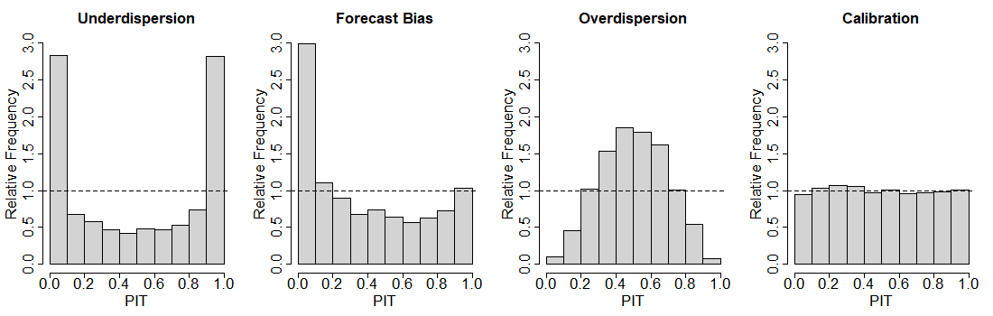
Fig. 86 Visual Assessment of Calibration of a Probabilistic Forecast via PIT Histograms.#

Another common tool to assess the qualitiy of a probilistic forecasts are so-called scoring rules, see, e.g. [Winkler, 1996] and [Gneiting and Raftery, 2007]. It is a mapping \(S(F,y)\) that assigns the probabilistic forecast \(F\) and the respective verifying observation \(y\) a value in \(\mathbb{R}\).

A popular scoring rule is the Continuous Ranked Probability Score (CRPS):

\[ \text{CRPS}(F,y) = \int_{- \infty}^{\infty} \; ( F(x) - \mathbb{I}_{\{x \geq y\}} )^2 \mathrm{d} x, \]

which essentially measues the (squared) difference between the predictive distribution \(F\) and the empirical distribution of the observations \(y\).

The CRPS can equivalently be represented as

\[ E_F | X - y | - \frac{1}{2} \; E_F | X - X' |, \]

where \(E_F\) denotes the expectation with respect to \(F\), \(X\) and \(X'\) are independent random variables with distribution \(F\).

This represation explains the popularity of the CRPS, as it shows that the CRPS measures both, calibration and sharpness within one score. The first expectation refers to the calibration part, it measures the consistency between the predictive distribution (represented by the random variable with the respective distribution) and the observation \(y\). The second expecation describes the spread of the predictive distribution (represented by the difference between two independent random variables coming from the same distribution \(F\)).

Apart from this appealing interpretational advante the CRPS is also a so-called proper scoring rule [Gneiting and Raftery, 2007], a property that encourages the use of the true distribution as forecasting distribution.

References#

Bje04: V. Bjerknes. Das Problem der Wettervorhersage, betrachtet vom Standpunkte der Mechanik und der Physik. Meteorologische Zeitschrift. Ed. Hölzel, 1904.
Gne08: T. Gneiting. Editorial: probabilistic forecasting. Journal of the Royal Statistical Society Series A, 171:319–321, 2008.
GBR07: T. Gneiting, F. Balabdaoui, and A. E. Raftery. Probabilistic forecasts, calibration and sharpness. Journal of the Royal Statistical Society Series B, 69:243–268, 2007.
GK14: T. Gneiting and M. Katzfuss. Probabilistic forecasting. Annual Review of Statistics and Its Application, 1:125–151, 2014.
GR05(1,2): T. Gneiting and A. E. Raftery. Weather forecasting with ensemble methods. Science, 310:248–249, 2005.
GR07(1,2): T. Gneiting and A. E. Raftery. Strictly proper scoring rules, prediction, and estimation. Journal of the American Statistical Association, 102:359–378, 2007.
GRWIG05: T. Gneiting, A. E. Raftery, A. H. Westveld III, and T. Goldman. Calibrated probabilistic forecasting using ensemble model output statistics and minimum CRPS estimation. Monthly Weather Review, 133:1098–1118, 2005.
HC97: T.M. Hamill and S.J. Colucci. Verification of eta–rsm short-range ensemble forecasts. Monthly Weather Review, 125:1312–1327, 1997.
Kal03: E. Kalnay. Atmospheric Modelling, Data Assimilation and Predictability. Cambridge University Press, 2003.
LP08: M. Leutbecher and T. N. Palmer. Ensemble forecasting. Journal of Computational Physics, 227:3515–3539, 2008.
Lor63: E. N. Lorenz. Deterministic nonperiodic flow. Journal of the Atmospheric Sciences, 20:130–141, 1963.
Pal02: T. N. Palmer. The economic value of ensemble forecasts as a tool for risk assessment: from days to decades. Quarterly Journal of the Royal Meteorological Society, 128:747–774, 2002.
RGBP05: A. E. Raftery, T. Gneiting, F. Balabdaoui, and M. Polakowski. Using Bayesian model averaging to calibrate forecast ensembles. Monthly Weather Review, 133:1155–1174, 2005.
VBD+21(1,2): S. Vannitsem, J.B. Bremnes, J. Demaeyer, G.R. Evans, J. Flowerdew, S. Hemri, S. Lerch, N. Roberts, S. Theis, A. Atenica, Z.B. Bouallègue, J. Bhend, M. Dabernig, L. De Cruz, L. Hieta, O. Mestre, L. Moret, I.O. Plenković, M. Schmeits, M. Taillardat, J. Van den Bergh, B. Van Schaeybroeck, K. Whan, and J. Ylhaisi. Statistical postprocessing for weather forecasts – review, challenges and avenues in a big data world. Bulletin of the American Meteorological Society, 102:E681–E699, 2021. doi:https://doi.org/10.1175/BAMS-D-19-0308.1.
VWM18: S. Vannitsem, D. Wilks, and J. W. Messner. Statistical postprocessing of ensemble forecasts. Elsevier, 2018.
WH07: D. Wilks and T. M. Hamill. Comparison of ensemble-MOS methods using GFS reforecasts. Monthly Weather Review, 135:2379–2390, 2007.
Win96: R. L. Winkler. Scoring rules and the evaluation of probabilities. Test, 5:1–60, 1996.

Authors#

Annette Möller