Distribution Functions

Part of a series: Stochastic fundamentals.

Follow reading here

Definitions and elementary properties

Random variables are typically characterized by distribution functions. These functions describe the probability that the random variable assumes a given value (discrete case) or falls in a certain interval (continuous case). We define and discuss these distribution functions starting from the discrete case.

The probability mass function (PMF)

Let \((\Omega, \Sigma, P)\) be a probability space and \(X:\Omega \longrightarrow E \subset \mathbb{R}\) a discrete random variable (\(E\) is countable). Then the probability mass function \(f_x : E \longrightarrow [0,1]\) is defined as: \(\label{eq:prob_mass_func} f_X(x) = P(X=x) = P(\{ \omega \in \Omega : X(\omega) = x\})\)

Example The probability mass function of a fair die is given by: \(f_X(i) = \frac{1}{6} \quad \mbox{where} \ i \in \{1,2,3,4,5,6\}\)

The cumulative distribution function (CDF)

Let \(X: \Omega \longrightarrow \mathbb{R}\) be a continuous random variable. The cumulative distribution function (CDF) is defined as \(\label{eq:cdf_def} F_X(x) = P(X\leq x) = P(\{ \omega \in \Omega : X(\omega) \leq x\}),\) i.e. the probability that \(X\) assumes a value smaller than \(x\).

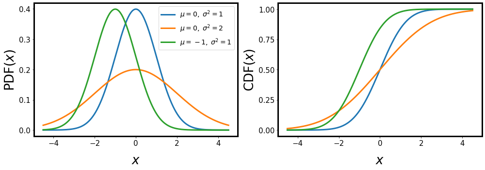
Fig. 11 PDF and CDF for different values for the mean \(\mu\) and variance \(\sigma^2\).

Properties

• Using the CDF, we can directly give the probability that the random variable \(X\) falls in a certain interval: \(P(a < X \leq b) = F_X(b) - F_X(a)\)

• The CDF \(F_X\) is non-decreasing and right-continuous, i.e. \(\lim_{s \rightarrow t} F_X(s) = F_X(t)\)

• The CDF has the limiting values

  \(\begin{split} \lim_ {s \rightarrow -\infty} F_X(s) &= 0 \\ \lim_ {s \rightarrow +\infty} F_X(s) &= 1. \end{split}\)

The probability density function (PDF)

Let \(X: \Omega \longrightarrow \mathbb{R}\) be a continuous random variable. Then \(X\) has the probability density function (PDF) \(f_X:\mathbb{R} \longrightarrow \mathbb{R}\) if \(P(a \leq X \leq b) = \int_a^b f_X(x) \ dx\) Hence, the CDF is given by \(F_X(x) = \int_{-\infty}^{x} f_X(u) \ du\) and, if the PDF \(f_X\) is continuous at \(x\), then: \(f_X(x) = \frac{d}{dx} F_X(x)\)

Comments CDFs are more “well-behaved” and exist for all random variables \(X: \Omega \longrightarrow \mathbb{R}\), hence mathematicians tend to prefer CDFs to PDFs. Physicists, on the other hand, tend to prefer working with PDFs since they are more intuitive in a sense that \(f_X(x) dx\) is interpreted as the probability that \(X\) assumes a value in the interval \((x, x+dx)\).

Consider for example the CDF \(\begin{aligned} F_X(x) = \left\{ \begin{array}{l l l} 0 && x < 0 \\ \frac{1}{2} + \frac{x}{2} \; & \mbox{for} \; & 0 \le x \le 1 \\ 1 && 1 < x . \end{array} \right. \end{aligned}\)

which can be interpreted as follows. The random variable \(X\) either assumes the value zero with probability \(\frac{1}{2}\) or a value drawen uniformely at random from the the interval \([0,1]\), also with probability \(\frac{1}{2}\).

If we want to derive a PDF, we would obtain

\(\begin{aligned} f_X(x) = \frac{1}{2} \delta(x) + \left\{ \begin{array}{l l l} 0 && x < 0 \\ \frac{1}{2} \; & \mbox{for} \; & 0 \le x \le 1 \\ 1 && 1 < x . \end{array} \right.\end{aligned}\) with the Dirac \(\delta\)-function.

This is of course no longer a proper function and hence should not be called a PDF. Nevertheless, this notation is regularly used among physicists.

Transformation of Variables

We will often encounter situations where we consider functions of random variables. These functions are again random variables since they also map from \(\Omega\) to \(\mathbb{R}\) and we can also assign probabilities – more precisely distribution functions – to these quantities. Here we show how the distributions functions are transformed.

So let \(X: \Omega \rightarrow \mathbb{R}\) be a continuous random variable with CDF \(F_X(x)\), PDF \(f_X(x)\) and \(g: \mathbb{R}\) an invertible function. The random variable \(Y:=g(X)\) has the distribution

\[\begin{split} F_Y(y) &= \left\{ \begin{array}{l l} F_X(g^{-1}(y)) & \mbox{if g is monotonically increasing} \\ 1- F_X(g^{-1}(y)) \; & \mbox{if g is monotonically decreasing}. \end{array} \right. \\ f_Y(y) &= \frac{1}{|g'(g^{-1}(y))|} \; f_X(g^{-1}(y)) . \end{split}\]

We proof this statement starting from the CDF. From the definition we find

\[ F_Y(y) = P(Y \le y) = P( g(X) \le y ). \]

Now if \(g\) is monotonically increasing this can be rewritten as

\[\begin{split} F_Y(y) &= P( g(X) \le y ) \\ &= P(X \le g^{-1}(y) ) \\ &= F_X(g^{-1}(y)) \end{split}\]

If \(g\) is monotonically decreasing we find instead

\[\begin{split} F_Y(y) &= P( g(X) \le y ) \\ &= P(X \ge g^{-1}(y) ) \\ &= 1- F_X(g^{-1}(y)). \end{split}\]

The PDF is found by taking the derivative of the CDF taking care of the chain rule and the inverse function theorem. For a monotonically increasing \(g\) we have

\[\begin{split} f_Y(y) &= \frac{d}{dy} F_Y(y) = \frac{d}{dy} F_X(g^{-1}(y)) \\ &= f_X(g^{-1}(y)) \frac{d g^{-1}(y)}{dy} \\ &= f_X(g^{-1}(y)) \, \frac{1}{g'(g^{-1}(y))} \, . \end{split}\]

For a monotonically decreasing \(g\) we have

\[\begin{split} f_Y(y) &= \frac{d}{dy} F_Y(y) = \frac{d}{dy} \left[ 1- F_X(g^{-1}(y)) \right] \\ &=- f_X(g^{-1}(y)) \frac{d g^{-1}(y)}{dy} \\ &= f_X(g^{-1}(y)) \, \frac{-1}{g'(g^{-1}(y))} \, , \end{split}\]

which concludes the proof.

Authors

Philipp Böttcher, Dirk Witthaut