Normal Distribution#
Part of a series: Stochastic fundamentals.
Follow reading here
Definition:#
A random variable \(X\) is normally distributed with mean \(\mu\) and variance \(\sigma\) if its PDF is given by
We write \(X \sim N\).
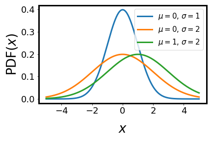
Fig. 12 Normal distributions with different values for the mean \(\mu\) and standard deviation \(\sigma\).#
Properties:#
\(E(X) = \mu\)
The higher moments are given by \(E[(X-\mu)^2]=\begin{cases} 0 & \text{if p is odd}\\ \sigma^p(p-1)!! & \text{if p is even} \end{cases}\)
Here \((p-1)!! = (p-1)(p-3)(p-5)...1\) is the double factorial
The CDF is given by \(F_X(x) = \Phi \left( \frac{x-\mu}{\sigma}\right) = \frac{1}{2}\left[1 + \text{erf}\left(\frac{x-\mu}{\sqrt{2}\sigma}\right) \right]\) with the special functions \(\Phi (x) = \frac{1}{\sqrt{2 \pi}} \int_{-\infty}^x e^{-t^2/2} \ dt\)
\(\text{erf} (x) = \frac{1}{\sqrt{ \pi}} \int_{-x}^{+x} e^{-t^2} \ dt\)
The 68-95-99.7 rule (3-\(\sigma\)-rule)
How probable is it that \(X\) assumes a value which differs from \(\mu\) less than \(n \cdot \sigma\)?
\[P(|x-\mu| \leq n\sigma ) = F_X(\mu+n \sigma) - F_X(\mu-n \sigma) :\]\[n=1 \quad : \quad 0.683...\]\[n=2 \quad : \quad 0.954...\]\[n=3 \quad : \quad 0.997...\]
Why are normally distributed random variables so important in maths and physics?
Many variables are really normally distributed.
Example: Position of a quantum harmonic oscillator in its ground state
Adding up many iid random variables (with finite variance), the sum tends to a normally distributed random variable.
This is called the central limit theorem, which we prove explicitly later.
Thus: Many uncorrelated stochastic influences
\(\Rightarrow\) Cumulated stochastic influence is normal.
Of all distributions with fixed expectation values \(E(X)=\mu\) and fixed variance \(V(X)=\sigma^2\), the normal distribution \(N(\mu,\sigma^2)\) is the one with maximum entropy \(H(X)= \int_{-\infty}^{+\infty} f_X(x) \log \left(f_X(x)\right) dx \ .\) Thus, if we have only \(\mu\) and \(\sigma^2\) and otherwise have maximum uncertainty about \(X\), we should assume that it’s normal.
Convenience
Large deviations are exponentially rare
All integrals \(\int dx f_X(x) g(x)\) converge
All moments exist and are analytically known
We can also extend this definition to the multivariate case.
So consider a set of \(k\) random variables \(X_j: \Omega\rightarrow\Re^k\) for all \(j=1...k\). Defining component-wise addition and scalar multiplication, we can call the set of random variables a random vector $\vec{x} =
Def. A random vector \(\vec{X}\) is (multivariate) normally distributed with mean \(\vec{\mu} \in \Re ^{k\times k}\) and covariance matrix \(S\in \Re ^{k\times k}\) if it has the PDF \(f_{\vec{X}}(\vec{x})=\frac{1}{\sqrt{2\pi}^k\sqrt{\det(S)}} e^{-\frac{1}{2}(\vec{x}-\vec{\mu})^TS^{-1}(\vec{x}-\vec{\mu})}\) We write \(\vec{X} \sim N(\vec{\mu},S)\)
Lemma A random vector \(\vec{X}:\Omega\rightarrow \Re ^k\) is normally distributed if and only if any linear combination \(\Sigma ^k_{j=1} a_j \vec{X_j}\) is (univariate) normally distributed.