Conditional Probabilities#
Part of a series: Stochastic fundamentals.
Follow reading here
Introductory example#
As an introductory example to the field of conditional probabilities we consider a topical problem in public health: Antigen tests for the new Corona virus. The tests can be completed and evaluated much more rapidly than more elaborate PCA test, but are known to be less reliable. So consider a person who has completed such an antigen test and received a positive result. This is a strong hint that the person is infected but as mentioned above the test is not perfect. So what is the probability that the person is infected now? This is a conditional probability, conditioned on the outcome of the antigen test. We will further elaborate this example at the end of this chapter after providing a formal definition.
Definition#
Let \((\Omega, \Sigma, P)\) be a probability space. Now assume that \(\omega \in \Omega\) is such that an event \(B\) has already occurred, i.e, \(\omega \in B\). We call \(B\) a condition. Now consider a second event \(A \in \Sigma\). The probability for the event \(A\) given that \(B\) has already occurred is called the conditional probability and expressed as \(p(A | B)\). We illustrate the relation of the sets \(A\) and \(B\) in the figure below.

Fig. 5 The condition \(B\) is assumed to be satisfied. Loosely speaking, we thus know that we “restrict ourselves to the right part” of the initial set of outcomes \(\Omega\).#
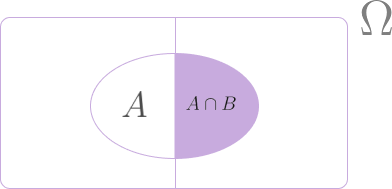
Fig. 6 The conditional probability \(P(A\) | \(B)\) is the probability that the event \(A\) occurs given the event \(B\) has already occurred. It is equal to the probability of finding both \(A\) and \(B\) relative to probability of finding \(B\).#
Definition Let \(A, B \in \Sigma\) and \(p(B) > 0\). The joint probability of \(A\) and \(B\) is defined as \(P(A \cap B) = P(\{\omega \in A \} \ \mbox{and} \ \{\omega \in B \})\)
The conditional probability is defined as \(P(A|B) = \frac{P(A \cap B)}{P(B)}\)
Bayes’ Theorem#
Bayes’ theorem states that \(\label{eq:bayes_thm} P(A|B) = \frac{P(B|A) P(A)}{P(B)} \, .\)
Proof. The joint probability of \(A\) and \(B\) is \(P(A \cap B) = P(B \cap A)\). So from the definition of conditional probability, \(P(A|B) P(B) = P(B|A) P(A)\).
Corollary Let \(A_1, A_2, \ldots, A_s\) be pairwise disjoint events, i.e, \(A_j \cap A_k = \emptyset, \ \forall \ \mbox{pairs} \ j, k\). Let \(P(A_j) > 0, \ \forall \ j = 1,2, \dots, s\), and \(\begin{aligned} \bigcup _{j=1} ^{s} A_j = \Omega \, \end{aligned}\) (this is called a decomposition of \(\Omega\)).
Then we can express the probability of another event \(B\) as \(\begin{aligned} P(B) = \sum _{j=1} ^s P(B|A_j) \ P(A_j) \, . \end{aligned}\)
The example (continued)#
Let us now continue with our introductory example from the previous entry and elaborate this with numbers using Bayes’ theorem. Our initial question was: What is the probability that a person is infected conditioned on the positive outcome of an antigen test. To formalize this question we define two events:
\(I\): A person is infected.
\(T\): A person receives a positive test result.
Our initial question is thus: What is the conditional probability \(P(I | T)\).
To answer this question, we need some facts about the antigen test itself. Following a publication of the Robert Koch institute (link), we assume the following properties:
If a person is truly infected, the test will yield the correct positive result with a probability of \(P(T|I) = 0.8\). This is called the sensitivity.
If a person is not infected, the test will yield the correct negative result with a probability of \(P(\bar T|\bar I)=0.98\). This is called the specificity.
We now use Bayes’ theorem in the form \(\begin{aligned} P(I|T) = \frac{P(T|I) P(I)}{P(T)} \end{aligned}\)
We then eliminate \(P(T)\) in the above expression using the decomposition corollary above, \(\begin{aligned} P(T) &= P(T|I) P(I) + P(T|\bar I) P(\bar I) \\ &= P(T|I) P(I) + \left[1 - P(\bar T | \bar I) \right] \times \left[1 - P(I) \right]. \end{aligned}\)
Now the answer to the initial question depends on the actual number of infected persons. If it is very high at \(10\%\), we find
\(\begin{aligned} P(I) = 0.1 \quad \Rightarrow \quad P(I|T) \approx 0.82. \end{aligned}\)
Hence, a positive test implies an infection with a high probability of above \(80\%\). If it is very low, say \(0.05\%\), then we find instead
\(\begin{aligned} P(I) = 0.0005 \quad \Rightarrow \quad P(I|T) \approx 0.02. \end{aligned}\)
That is, the probability of being infected is only \(2\%\) even in the case of a positive test.
The above calculations can also be visualized using a decision tree as in the figure below.

Fig. 7 Interpreting an antigen test for the new Corona virus. (a) Scenario with a very low infection rate of just 5 out of 10000 persons. A positive test implies an infection with the probability \(P(I|T) = \frac{P(I \cap T)}{P(T)} = \frac{4}{204} \approx 2\%\). (b) Scenario with a very high infection rate of 1000 out of 10000 persons. A positive test implies an infection with the probability \(P(I|T) = \frac{P(I \cap T)}{P(T)} = \frac{800}{980} \approx 82\%\). This figure is a recreation and translation of the information found in informational material found on the RKI webpage.#