Expected Value, Variance and Higher Order Moments#
Part of a series: Stochastic fundamentals.
Follow reading here
The expected value#
Introduction#
Expected values were first discussed in the context of gambling by Christian Huygens in his paper “Van rekeningh in spelen van geluck” published in 1656 [Huygens, 1895]. So let’s follow this approach and look at a game of chance and model it as a stochastic experiment. We consider a wheel of fortune with sectors \(\omega_1,\omega_2,\ldots, \omega_s\). If the pointer stops at a sector \(\omega_j\) (which happens with a probability \(P(\{\omega_j\})\)), you win an amount of money \(X(\omega_j)\). What would you be willing to pay to play such a game, assuming that you are risk-neutral?
Answering this question directly leads to the definition of the expected value. The expected value of the return, which is given by
and a risk-neutral person would pay at most this amount of money to join the game. Let us now formalize this description.
Definition#
Let \(X: \Omega \longrightarrow \mathbb{R}\) be a random variable. If \(\Omega\) is countable, the expected value of \(X\) is defined as \(E(X) = \sum _{\omega \in \Omega} X(\omega) \ P(\{\omega\})\) If \(\Omega\) is uncountable, then the expected value is defined as \(E(X) = \int _{\Omega} X(\omega) \ P(d\omega). \label{eq:def-expect-continuous}\)
Some properties#
Let us summarize some important properties of the expected value. So let \(X\) and \(Y\) be random variables, \(a \in \mathbb{R}\) and \(A \in \Sigma\) be an event. The expected value \(E\) has the properties
\(E(X+Y) = E(X) + E(Y)\)
\(E(aX) = a E(X)\)
\(E(\mathbf{1}_A) = P(A)\) where \(\mathbf{1_A}\) is the indicator function.
\(X \leq Y\) , i.e \(X(\omega) \leq Y(\omega) \ \forall \omega \in \Omega\) implies \(E(X) \leq E(Y)\).
Expected values, PDFs and the transformation rule#
In many important applications, we characterize a random variable not directly by the mapping \(X: \Omega \longrightarrow \mathbb{R}\) but in terms of its distribution functions. In this case, we can compute the expected value of \(X\) or any function of \(X\) directly from the PDF.
So let \(X\) be a random variable with the PDF \(f_X(x)\) and \(g: \mathbb{R} \longrightarrow \mathbb{R}\) an arbitrary function. Then the expected value of the transformed random variable \(g(X)\) is given by \(E(g(X)) = \int_{-\infty}^{+\infty} f_X(x) \ g(x) \ dx.\) In particular, choosing \(g\) as the identity, we get \(E(X) = \int_{-\infty}^{+\infty} f_X(x) \ x \ dx.\)
The Variance#
Definition.#
The variance \(V(X)\) of a random variable \(X: \Omega \longrightarrow \mathbb{R}\) is defined as \(V(X) = E \{ [X - E(X)]^2 \}\). The variance of \(X\) is also expressed as \(\sigma^2(x)\) or \(\sigma_x^2\). The square root of the variance, \(\sigma(X) = \sqrt{V(X)}\) is called the standard deviation.
Some properties of the variance#
\(V(X) = E((X-a)^2 ) - (E(X)-a)^2 \quad \forall a \in \mathbb{R} \quad \mbox{(Steiner formula)}\)
\(V(X) = E(X^2 ) - (E(X))^2\)
\(V(X) = \min_{a\in \mathbb{R}} \ (E(X-a))^2\)
\(V(a X + b) = a^2 \ V(X) \quad a,b \in \mathbb{R}\)
\(\begin{split} V(X) &\geq 0 \\ \mbox{and} \quad V(X) &= 0 \implies P(X=a) = 1 \quad \mbox{for one value} \ a\in \mathbb{R} \end{split}\)
Standardization of a random variables#
Let \(X\) be a random variable with \(V(X)>0\). Recall that \(V(X)=0\) implies that \(P(X=a)= 1\) for some \(a \in \mathbb{R}\). This corresponds to a sure outcome of a stochastic experiment – a boring situation which we exclude here.
Now let us define the random variable \(X^*\) as \(X^* = \frac{X - E(X)}{\sigma(X)}\). Then, we have \(E(X^*) = 0\) and \(V(X^*)=1.\)
The new random variable \(X^*\) is called the standardisation of \(X\). Its distribution functions (PDF and CDF) have the same shape as for the original random variable, but are shifted and stretched. This procedure simplifies the comparison of the distribution of different random variables.
The Tschebychev inequality#
The expected value reflects our expectation about the value of a random variable in a stochastic experiment. However, deviations from the expected value in actual realization can be quite large, depending on the higher moments of random variable. The Tschebychev inequality now provides a general upper bound for the the probability of finding large deviations.
So let \(X: \Omega \rightarrow \mathbb{R}\) be a real random variable. For every \(\epsilon>0\) we have \( P\left( \left| X - E(X) \right| \ge \epsilon \right) \le \frac{V(X)}{\epsilon^2} \, \).
Before we proof this statement, we have a few remarks
The Tschebyschev inequality assures that “large deviations” from the expected value \(E(X)\) are rare. How rare depends on the variance of the random variable \(V(X)\).
The value of the inequality lies in its generality – it applies for all random variables independent of its actual distribution and provides a bound which vanishes algebraically with \(\epsilon\). For many distributions of practical importance one can get much sharper bounds that actually decrease exponentially with \(\epsilon\).
In fact, there is a subfield of probability theory devoted to the study of large deviation and we will provide a very short introduction in chapter Large deviation theory.
Proof of the Tschebychev inequality#
Define the functions \(g,h: \mathbb{R} \rightarrow \mathbb{R}\) as
which are illustrated in figure below. We then have
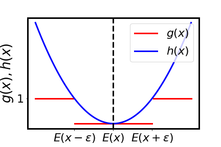
Fig. 8 Illustration of the function \(g(X)\) and \(h(X)\) used in the proof of the Tschebychev inequality.#
We can now use indicator functions to proof the actual result:
Higher moments#
Sometimes one also needs the higher moments of a random variable, which are defined as
for any natural number \(n\in \mathbb{N}_{+}\). The third and fourth moment are particularly useful to characterize the shape of a probability distribution. In this case one typically uses the moments of the standardized random variable to disentangle the impact of the position and scale of the distribution from its shape.
Skewness#
Let \(X*\) be the standardisation of \(X\). Then the standardised 3rd moment, \(E(X^{*3})\) measures the skewness of a probability distribution. This parameter is often used to describe if the distribution is symmetric or skewed to low or highvalues of \(x\) as illustrated in the following figure.
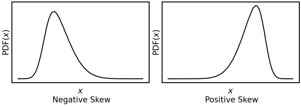
Fig. 9 Positive and negative skewness of probability distributions.#
Kurtosis#
The Kurtosis \(\kappa\) or the standardised 4th moment \(E(X^{*4})\) measures the importance of outliers (i.e. events with \(X\geq \sigma\)). High kurtosis is found if,
there is some probability for extreme outliers or
the probability density is concentrated in the tail.
In older references, kurtotsis is sometimes interpreted as peakedness, but this interpretation not correct, cf. [Westfall, 2014]. In practice, one often compares the kurtosis to that of a normal distribution with a Gaussian PDF leading to the following classification:
Normal distribution for \(E(X^{*4})=3\)
Super-Gaussian distributions for \(E(X^{*4})>3\) (Example: Poisson distribution)
Sub-Gaussian distributions for \(E(X^{*4})<3\) (Example: Uniform distribution).
Instead of the kurtosis, the excess kurtosis \(\kappa\) (kurtosis minus 3) is often used to explicitly contrast the considered distribution with the normal distribution.
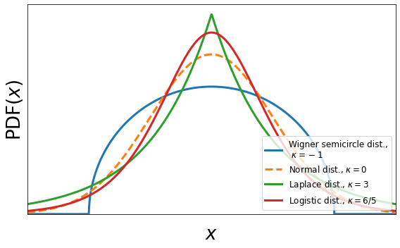
Fig. 10 Excess kurtosis \(\kappa\) for different distribution that all have a variance of 1.#