Scenario Generation and Validation in Renewable Power Generation#
Part of a series: Uncertainty in Future Energy Systems.
Follow reading here
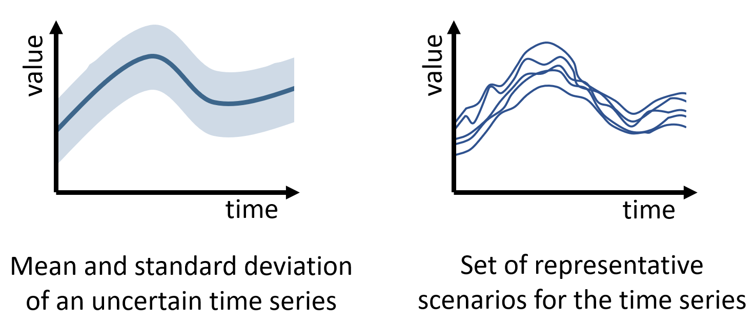
Fig. 53 An uncertain time series is a time-dependent uncertain parameter. If known, the uncertainty in the time-dependent parameter can be described by its mean and standard deviation (left). Alternativly, the uncertainty can be represented by a set of discrete scenarios (right). These scenarios can be based on historical data, sampled from the probability distribution function if it is known, or generated, e.g., by deep generative models.#
The following overview is based on [Cramer et al., 2022] that is referred to for more details and explanation.
Energy time series are key for the operation and design of energy systems. For example, a time series of renewable energy generation and electricity load within an energy community can be used to optimally operate and design an energy storage. Uncertainty connected to the time series can be represented by means of scenarios, i.e., time series that represent possible realizations of an uncertain time-dependent parameter (Fig. 53). Thus, a set of scenarios is a discrete approximation of a multi-dimensional probability distribution. These scenarios can be used to account for uncertainty when optimizing the operation and design of an energy system.
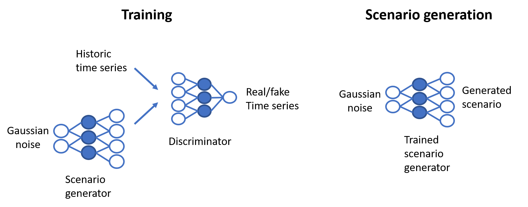
Fig. 54 Neural networks can be used to learn the probability distribution of historical time series and generate new scenarios. The training (left) is shown exemplarily for a so-called generative adversarial network. Here, a network generates scenarios from Gaussian noise. The goal is that the first network learns to generate “real” scenarios. For this purpose, a second network, i.e., a discriminator, is used to distinguish real and fake scenarios. For the scenario generation (right), the trained scenario generator can be used to generate new scenarios from Gaussian noise.#
Typically, the probability distributions of energy time series are unknown and can be influenced by many factors, e.g., weather, seasonality, day-time, and location. Recorded time series represent historical realizations of the uncertain parameter and can be used to understand the underlying probability distribution. Neural networks can learn the probability distributions of historical data and generate representative sets of scenarios [Chen et al., 2018], which is exemplarily shown in Fig. 54. Here, the neural network is trained such that it can transform a sample of a Gaussian distribution to a time series scenario. Hence, a realization of the known Gaussian distribution is transformed to a realization of the unknown probability distribution of the time series. Using different samples of the Gaussian distribution generates a representative set of scenarios. Neural networks for scenario generation include generative adversarial networks (GAN) [Goodfellow et al., 2020], Wasserstein-GANs (WGAN) [Arjovsky et al., 2017], Variational Autoencoders (VAE) [Kingma and Welling, 2013], and Normalizing Flows [Papamakarios et al., 2019]. The methods differ in network structure and loss function, but follow the same principle for final scenario generation, i.e., using Gaussian samples as input and returning a vector with fixed size, i.e., a time series scenario.
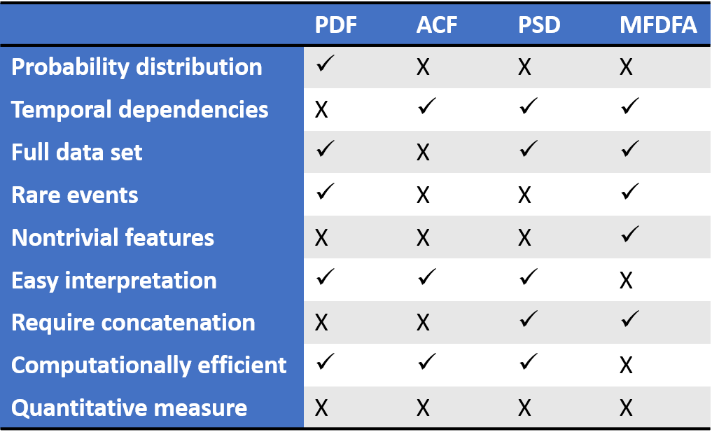
Fig. 55 Vaious methods can be used to validate generated scenarios. The table shows the differences between the methods and is taken from [Cramer et al., 2022]. Each method can be used to evaluate certain characteristics and properties of the generated scenarios. We refer to [Cramer et al., 2022] for a more detailed explanation.#
With the use of scenario generation methods, scenario validation methods become imperative in order to judge the quality of the generated scenarios. In general, various methods can be applied to the original data set and the generated data set in order to compare the sets. If the original and generated data show similar results based on the proposed methods, the quality of the generated scenarios can be validated. Fig. 55 shows a comparison of the methods and the respective characteristics and properties that can be checked by them. A combination of methods should be used to evaluate the quality of scenarios [Cramer et al., 2022], i.e., probability density function (PDF) [Davis et al., 2011, Parzen, 1962], autocorrelation function (ACF) [Stoica et al., 2005], power spectral density (PSD) [Stoica et al., 2005], and multifractal detrended fluctuation analysis (MFDFA) [Salat et al., 2017]. PDF of the historical and the generated data can be estimated by means of a kernel density estimation. Here, a comparison both on linear and logarithmic scale should be done. ACF describes the correlation of the time series between time steps. Generated scenarios can have a similar Pearson correlation, i.e., the normalized auto-covariance, as the historical data. However, this does not indicate a good representation of the true auto-correlation within the full historical data set. Furthermore, different stochastic processes can have similar ACF values. Thus, ACF should not be used as an exclusive approach. PSD can be used to analyze periodic behavior and is based on Fourier transforms that return the amplitude for possible frequencies in the data. These amplitudes are squared to obtain the PSD. PSD can be additionally smoothed by means of the Welch’s method [], i.e., overlapping segments of the time series. Frequencies of up to half the length of the scenarios should be considered. MFDFA can be used to identify peaks, burst and plateaus in the data and analyzes data relative to the sampling rate. Here, the change in fluctuation behavior is analyzed by means of the Hurst exponent. For an example of the MFDFA and a detailed explanation on the Hurst exponent, we refer to the fluctuations and uncertainty of solar power generation. Note that these methods are based on visual inspection and thus can potentially lead to subjective interpretation.
References:#
- ACB17
Martin Arjovsky, Soumith Chintala, and Léon Bottou. Wasserstein GAN. arXiv e-prints, jan 2017. URL: http://arxiv.org/abs/1701.07875, arXiv:1701.07875.
- CWKZ18
Yize Chen, Yishen Wang, Daniel Kirschen, and Baosen Zhang. Model-Free Renewable Scenario Generation Using Generative Adversarial Networks. IEEE Transactions on Power Systems, 33(3):3265–3275, may 2018. URL: http://ieeexplore.ieee.org/document/8260947/, arXiv:1707.09676, doi:10.1109/TPWRS.2018.2794541.
- CGM+22(1,2,3,4)
Eike Cramer, Leonardo Rydin Gorjao, Alexander Mitsos, Benjamin Schafer, Dirk Witthaut, and Manuel Dahmen. Validation Methods for Energy Time Series Scenarios From Deep Generative Models. IEEE Access, 10:8194–8207, 2022. doi:10.1109/ACCESS.2022.3141875.
- DLP11
Richard A. Davis, Keh-Shin Lii, and Dimitris N. Politis. Remarks on Some Nonparametric Estimates of a Density Function. In Selected Works of Murray Rosenblatt, pages 95–100. Springer New York, New York, NY, 2011. URL: http://link.springer.com/10.1007/978-1-4419-8339-8_13, doi:10.1007/978-1-4419-8339-8_13.
- GPAM+20
Ian Goodfellow, Jean Pouget-Abadie, Mehdi Mirza, Bing Xu, David Warde-Farley, Sherjil Ozair, Aaron Courville, and Yoshua Bengio. Generative adversarial networks. Commun. ACM, 63(11):139–144, oct 2020. URL: https://doi.org/10.1145/3422622, doi:10.1145/3422622.
- KW13
Diederik P Kingma and Max Welling. Auto-Encoding Variational Bayes. arXiv e-prints, dec 2013. URL: http://arxiv.org/abs/1312.6114, arXiv:1312.6114.
- PNR+19
George Papamakarios, Eric Nalisnick, Danilo Jimenez Rezende, Shakir Mohamed, and Balaji Lakshminarayanan. Normalizing Flows for Probabilistic Modeling and Inference. arXiv e-prints, dec 2019. URL: http://arxiv.org/abs/1912.02762, arXiv:1912.02762.
- Par62
Emanuel Parzen. On estimation of a probability density function and mode. The Annals of Mathematical Statistics, 33(3):1065–1076, 1962. URL: http://www.jstor.org/stable/2237880 (visited on 2022-10-16).
- SMA17
Hadrien Salat, Roberto Murcio, and Elsa Arcaute. Multifractal methodology. Physica A: Statistical Mechanics and its Applications, 473:467–487, 2017. URL: https://www.sciencedirect.com/science/article/pii/S0378437117300341, doi:https://doi.org/10.1016/j.physa.2017.01.041.
- SM+05(1,2)
Petre Stoica, Randolph L Moses, and others. Spectral analysis of signals. Volume 452. Prentice Hall, Inc., Upper Saddle River, New Jersey, USA, 2005.
Contributor#
Manuel Dahmen
Philipp Böttcher
Annette Möller