Inclusion of Temperature to Boost Markov Chain Monte Carlo#
Description#
Markov chain monte carlo (MCMC) offers a wide field of algorithms which share a common disadvantage: convergence speed. Several factors such as model complexity as well as initial and hyper-parameter values have an impact on the time until MCMC methods finally sample from the target distribution. Thus various approaches have been developed to tackle this issue, e.g. run independent Markov chains in parallel while allow them to switch states from time to time. Another way is to rescale the target function to make distributional peaks and valleys either more or less prominent. The following graphic shows the impact of differently scaled versions from the same target distribution. Introducing temperature into an MCMC setting equals scaling the target function in a certain way.
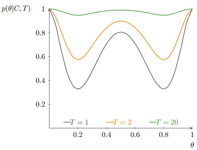
Fig. 32 The effect of scaling on a function.#
In a physical system, the temperature \(T \in [0,\infty)\)1 affects the state via \(\pi_T(\theta) \propto \exp(-\frac{1}{T} E(\theta))\). Here, \(E\) denotes the energy and is set to the negative log-posterior in Metropolis Hastings. The sampling distribution hence becomes \(\pi(\theta|X)^{\frac{1}{T}}\). The idea behind the usage of temperature is simple: The higher \(T\), the easier is an efficient exploration of the parameter space. This especially overcomes the challenges of deep local optima since they become less severe. When the temperature equals \(1\), the target distribution remains unscaled. Larger values flatten the surface, whereas \(T<1\) makes the distribution even peakier. Hence, the temperature is often bounded below by \(1\) in the context of MCMC.
One can restrict temperature to scale only the likelihood which is then referred to as thermodynamic integration.
Hence, a “hot” chain (i.e. \(T\to \infty, \tau \to 0\)) samples uniformly if the whole posterior is scaled or from the prior in thermodynamic integration, whereas a “cold” chain (i.e. \(T=1, \tau = 1\)) samples from the target distribution as usual.
Although the advantages seem appealing in theory, practical benefits heavily depend on how exactly temperature is included. Two approaches have become quite active research areas with that respect. Simulated annealing applies a specific schedule of temperatures onto a single Markov chain, whereas parallel tempering runs several independent chains with fixed individual temperatures.
Simulated Annealing#
The term annealing draws parallels to the mechanical process for the creation of crystalline structures in metals by alternation between high and low temperatures. This technique has been adapted to combinatorical problems some time ago [Kirkpatrick et al., 1983]. The idea is that the inclusion of a decreasing sequence of temperatures \(T_n\) shall reduce the costs of optimizations because the initial “hotter” distributions produce essentially the most flexible random search, whereas the “colder” ones point out local peaks and minima pretty clearly and get stuck to them.
To make this idea more precise, we recall the main idea of MCMC: A new proposal \(\theta^{(t)}\) is accepted if it yields a lower value of the target function. If the target function increases, the new proposal is accepted with the probability \(\exp\left[\pi(\theta^{(t)})/T_t-\pi(\theta^{(t-1)})/T_t\right]\). The main difference to ordinary MCMCs is that the temperature \(T_t\) now becomes a function of the step, too. The key challenge here, is the choice of an appropriate sequence of temperatures. One popular sequence is the geometric recursive scheme \(T_{t} = r \cdot T_{t-1} \ , r \in (0,1)\).
The following graphic emphasizes the impact of different simulated annealing schedules on three such Markov chains. Although the initial chain (orange) seems like a horizontal line, it is in fact moving through the space, but very slowly. A higher initial temperature and slower decrease factor \(r\) both increase the proposal variance in this particular case.
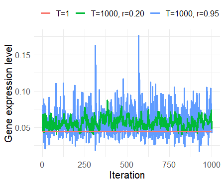
Fig. 33 Annealing of Markov chains.#
Furthermore, the example above highlights another important consequence of temperature on MCMC: The rescaling alters the limiting distribution. Therefore, simulated annealing samples are only reliable after the temperature schedule has converged. Consequently, a certain amount (depending on the starting temperature and \(r`\)) of initial samples must be discarded from subsequent analyses. The crucial question is whether this computational effort is outweighed by the improvement in performance (quicker traversing to high density areas and enhanced hyper-parameter adaption e.g. in the No-U-turn sampler).
Parallel Tempering#
Yet another quite common approach to utilize the benefits of temperature is parallel tempering (PT). It is best practice to not sample from one, but multiple chains with different initial values to arrive at more reliable estimates. Parallel tempering sets each of these chains up with a certain fixed temperature, e.g. as in the figure below. Hence, the chains are not equivalent, but quite similar for close temperatures. The trick is to allow state switching between neighboring chains after a specific number of iterations. It turns out that active mixing between temperatures benefits increased efficiency [Earl and Deem, 2005]. Nonetheless, an additional Metropolis acceptance step is required to manage the switching which makes PT computationally more intensive. This means for each potential exchange operation between two chains \(q,p\) the probability \(\min \left(1, \frac{\pi_q(\theta_p) \pi_p(\theta_q)}{\pi_q(\theta_q) \pi_p(\theta_p)} \right)\) must be calculated explicitly. The main advantage over simulated annealing is that PT fulfills the detailed balance condition and thus all the chains are time-reversible.
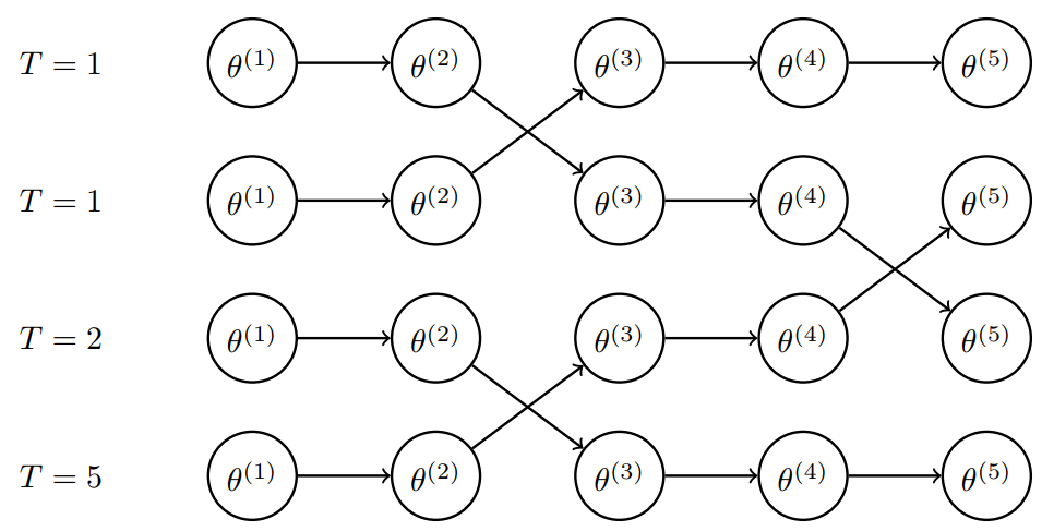
Fig. 34 Schematic representation of parallel tempered Markov chains.#
The main idea of PT it to allow the “colder” chains to still benefit from the efficient space exploration of their high-tempered counterparts. For the later calculation of summary statistics, only the cooler chains are considered. Nonetheless, PT comes hand in hand with other obstacles in form of new hyper-parameters. How many chains shall be drawn and which temperature values should be assigned? After how many iterations should the switching be performed? The modeller’s answers on these questions have a great impact on the chains behavior and convergence speed.
References#
Contributors#
Sonja Germscheid, Houda Yaqine, Dirk Witthaut, Kuan-Yu Ke
- 1
Please note that a synonymuous transformation exists and often found in literature which is called perk. These two share an inverse relationship with \(\tau = 1/T \in [0,1)\).