Choice of priors

In Bayesian statistics, we are interested in analyzing the posterior because it reflects what we have learnt from the collected data and the prior knowledge we chose. For large data sets, the posterior is more influenced by the likelihood, giving little room for the effect of the prior. In contrast, in the case of studies with a small amount of data, the prior choice has a significant impact on the posterior, and thus one has to be careful when choosing it.

In Bayesian methodology, we differentiate between two types of priors: informative priors and non-informative priors. As the names suggest, the informative prior reflects a clear prior knowledge of the parameter \(\theta\), while the non-informative prior reflects a very small to complete lack of prior knowledge.

Priors, in general, incorporate the amount of information we have about the model of the parameters before seeing the data. When researchers can specify a particular prior distribution favouring a range of values for the parameter over others, we say that they set an informative prior. The choice of a suitable informative prior can depend on several considerations, such as the findings of other similar studies (e.g. meta-analysis) or expert opinions. [1] gives a nice introduction to the topic of choosing priors for small samples research.

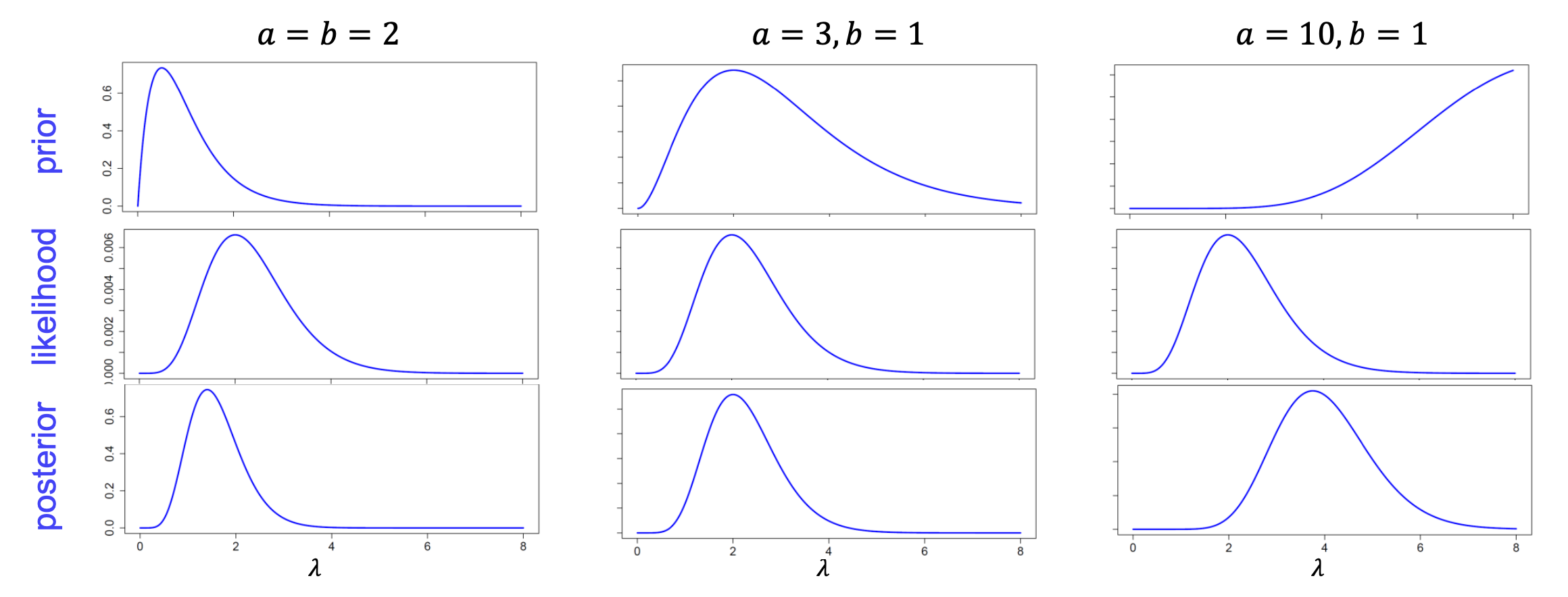
Fig. 26 Effect of informative priors on the posterior [copyright: Christiane Fuchs]

Depending on these considerations, one can have different prior distributions for other cases and models. When in particular the distributions of the posterior \(\pi(\theta|x_1,\dots,x_n)\) is of the same family as the prior distribution for the likelihood of the data, we say that the prior is a conjugate prior with respect to the likelihood. The advantage of this type of priors is mainly computational since we get a closed-form posterior distribution for which the posterior mean or other posterior statistics are analytically available. Conjugate priors can also be used in the settings where we don’t have a clear idea about which prior to use because they don’t require a lot of work, but again the choice of priors is relative to the statistician and not a hidden object.

Examples of conjugate priors

• Beta distribution is a conjugate prior with respect to a Bernoulli likelihood.

• Gamma distribution is a conjugate prior with respect to a Poisson likelihood.

If prior information about \(\theta\) is missing, alternative priors can be considered. Those latter are called non-informative priors.
There are several ways to construct such priors. The first prior that comes to mind is the uniform prior (or flat prior), which gives the same likelihood to each possible value of the parameter \(\theta\). Though it is straightforward, it has two downsides; the first is that the resulting posterior distribution is improper (i.e. does not define a density) when the parameter space is not compact. The second disadvantage is the variance under reparameterization, which creates a paradox. Under a reparameterization of \(\theta\), the prior on the new parameter still should reflect the no information property, but this is not the case. More precisely, if we do not have information about \(\theta\) we should not know anything about \(g(\theta)\), where \(g\) is a bijective function. But applying the change of variable rule:

\[ \pi(\theta)=U([0,1]),\ \phi=g(\theta) \leftarrow \pi(\phi)=|\frac{d}{d\phi}g^{-1}(\phi)| \]

gives instead to \(\phi=1/\theta\) the distribution

\[ \pi(\phi)=\pi(1/\theta))=1/\theta^2 \mathbb{1}_{[1,\infty)}(\theta) \]

This is contradictory, as \(\phi\) has no longer a non-informative prior.

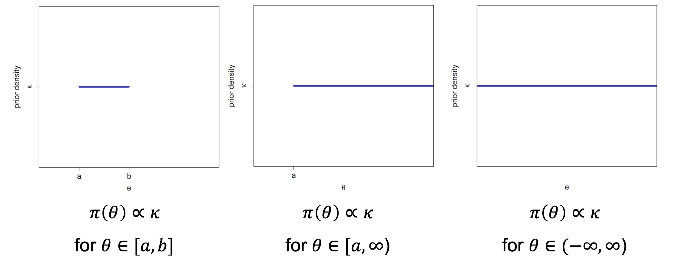
Fig. 27 Flat priors on different domains [copyright: Christiane Fuchs]

To overcome the issues coming from flat priors, Jeffreys introduced another type of priors called Jeffreys’ prior. Though it is known to be a non-informative prior in literature, it is not entirely non-informative. It is based on Fisher information, which represents the amount of information that can be brought by the model and the data about the parameter of interest \(\theta\). Therefore this prior reflects information directly from the sampling distribution, and it is defined by

\[ \pi(\theta)\propto I^{1/2}(\theta) \]

where \(I(\theta)\) is Fisher information given by

\[ I(\theta)=\mathbb{E}_\theta \left(\frac{\partial ^2 \log(\pi(x|\theta)) }{\partial \theta^2}\right) \]

The important feature of Jeffreys’ prior is the invariance under reparametrization, but it still has a downside and that is it does not satisfy the likelihood principle.

Lastly, we can mention another type of non-informative prior called the reference prior, and it maximizes the missing information in the experiment [Robert and others, 2007].

For more details about the choice and types of non-informative priors see [Bernardo, 1997].

References

Ber97

JM Bernardo. Noninformative priors do not exist: a discussion with josé m. Bernardo. J. Statist. Planning and Inference, 1997.

R+07

Christian P Robert and others. The Bayesian choice: from decision-theoretic foundations to computational implementation. Volume 2. Springer, 2007.

Authors

Houda Yaqine