Lévy Processes (DRAFT)

Part of a series: Stochastic fundamentals.

Follow reading here

An important class of stochastic processes is given by Lévy processes. They provide a flexible framework for processes with stationary and independent increments that allows for continuous processes as well as processes with jump discontinuities. For example, it encompasses well-known processes like Brownian motion and Poisson processes.

Definition

For the rest of this article, it is assumed that the underlying probability space is denoted by \((\Omega,\mathcal{F},\mathbb{P})\) and \(\mathbb{F}=(\mathcal{F}_t)_{t\ge0}\) is a filtration that is assumed to be right-continuous and complete.

An adapted stochastic process \(X=(X_t)_{t\ge0}\) on \(\mathbb{R}\) is a (one-dimensional) Lévy process if the following conditions are satisfied:

1. \(X_0=0~\mathbb{P}\)-almost surely.

2. For any \(n\in\mathbb{N}\) and \(0\le t_0<t_1<\dots<t_n<\infty\), the random variables \(X_{t_0},X_{t_1}-X_{t_0},\dots,X_{t_n}-X_{t_{n-1}}\) are independent.

3. \(X_{s+t}-X_s\stackrel{d}{=}X_t\) for \(0\le s,t<\infty\).

4. \(X\) is continuous in probability, i.e. for every \(t\ge0\) and \(\varepsilon>0\), it holds that

\[ \begin{align*} \lim_{s\to t}\mathbb{P}(|X_s-X_t|>\varepsilon)=0. \end{align*} \]

Condition 2 is called the “independent increments property”. It means that the behaviour of a Lévy process is independent along different time intervals. The “stationary increments property” 3 implies that, probabilistically, a process behaves equally in every time interval with the same length [Applebaum, 2009].

Properties

In this section, some characteristic properties of Lévy processes are collected [Protter, 2004].

• The characteristic function of a Lévy process \(X\) is determined by the so-called Lévy-Khintchine formula. For \(t\ge0\), it states that

  \[ \begin{align*} \phi_{X_t}(u)=\mathbb{E}\left[\mathrm{e}^{-\mathrm{i}uX_t}\right]=\mathrm{e}^{-t\psi(u)},\quad u\in\mathbb{R}, \end{align*} \]

  where the function \(\psi\colon\mathbb{R}\to\mathbb{C}\) is of the form

  \[ \begin{align*} \psi(u)=\frac{\sigma^2}{2}u^2-\mathrm{i}\gamma u+\int_{\mathbb{R}\setminus\{0\}}\left(1-\mathrm{e}^{-\mathrm{i}ux}+\mathrm{i}ux\mathbb{1}_{\{|x|<1\}}(x)\right)\nu(\mathrm{d}x), \end{align*} \]

  where \(\sigma\ge0,~\gamma\in\mathbb{R}\) and \(\nu\) is a measure on \(\mathbb{R}\setminus\{0\}\) satisfying

  \[ \begin{align*} \int_{\mathbb{R}\setminus\{0\}}(1\wedge x^2)\nu(\mathrm{d}x)<\infty. \end{align*} \]

  A Lévy process is uniquely characterised by its corresponding parameters \(\sigma,~\gamma\) and \(\nu\). In particular, \(\gamma\) describes the drift of such a process, \(\sigma\) represents the Brownian motion component and \(\nu\) is the Lévy measure determining jump intensities. The triplet \((\gamma,\sigma^2,\nu)\) is referred to as the generating triplet.

• Every Lévy process \(X\) can assumed to be càdlàg (i.e. the paths \(t\mapsto X_t\) are right-continuous \(\mathbb{P}\)-a.s. and the left limits exist \(\mathbb{P}\)-a.s.).1

• If there exists a constant \(C>0\) such that \(\sup_{0\le t<\infty}|\Delta X_t|<C\), where \(\Delta X_t=X_t-X_{t-}\) with \(X_{t-}=\lim_{s\uparrow t}X_s\), then \(\mathbb{E}[|X_t|^n]<\infty\) for every \(t\ge0\) and \(n\in\mathbb{N}\).

• Lévy processes are examples of Markov processes and semimartingales.

Examples

By concretely determining distributions for the stationary increments property 3, different kinds of Lévy processes arise [Bass, 2011, Applebaum, 2009]). Corresponding paths are depicted in Fig. 15.

Brownian Motion

One of the most prominent stochastic processes is Brownian motion. A process \(B=(B_t)_{t\ge0}\) is a Brownian motion if it is a Lévy process and if \(B_t\sim\mathcal{N}(0,t),~t\ge0\). It can also be seen as an example of a Markov process.

The generating triplet of a Brownian motion is given by \((\gamma,\sigma^2,\nu)=(0,1,0)\). In the context of Lévy processes, a Brownian motion \((B_t)_{t\ge0}\) exhibits some interesting path properties:

• The paths \(t\mapsto B_t\) are continuous \(\mathbb{P}\)-a.s.

• The paths \(t\mapsto B_t\) are \(\mathbb{P}\)-a.s. nowhere differentiable.

The continuity of the paths is a particular strong property since the paths of a Lévy process are in general only càdlàg.

Poisson Process

A Poisson process is a typical pure jump process whose name stems from the fact that the increments are Poisson distributed. More formally, a process \(N=(N_t)_{t\ge0}\) is said to be a Poisson process with parameter \(\lambda>0\) if it is a Lévy process and if \(N_t\sim Pois(\lambda t),~t>0\). Here, Poisson processes are discussed as examples of Markov processes.

The generating triplet is \((\gamma,\sigma^2,\nu)=(0,0,\lambda\delta_1)\), where \(\delta_x\) denotes the Dirac measure on \(\mathbb{R}\) for given \(x\in\mathbb{R}\). Furthermore, it can be shown that the paths of a Poisson process are increasing and constant except for jumps of size \(1~\mathbb{P}\)-a.s.

Compound Poisson Process

Compound Poisson processes are also pure jump processes, but they generalize Poisson processes by enabling processes to have arbitrary jump sizes.

For a mathematical definition, let \(N\) be a Poisson process with parameter \(\lambda>0\) and let \((Z_k)_{k\in\mathbb{N}}\) be a sequence of i.i.d. random variables taking values in \(\mathbb{R}\) with common law \(\mu_Z\), where \(\mu_Z\) is a distribution on \(\mathbb{R}\) with \(\mu_Z(\{0\})=0\). It is supposed that \(N\) is independent of all \(Z_k\)’s. A compound Poisson process \(Y=(Y_t)_{t\ge0}\) is then defined as

\[ \begin{align*} Y_t=\sum_{k=1}^{N_t}Z_k,\quad t\ge0. \end{align*} \]

The generating triplet of such a compound Poisson process is

\[ \begin{align*} (\gamma,\sigma^2,\nu)=\left(\lambda\int_{\{|x|<1\}}x\mu_Z(\mathrm{d}x),0,\lambda\mu_Z\right). \end{align*} \]

As already mentioned, the definition of a compound Poisson processes allows for random jump sizes. They can take all values supported by the distribution \(\mu_Z\). If \(\mu_Z=\lambda\delta_1\), for \(\lambda>0\), a compound Poisson process reduces to a Poisson process with parameter \(\lambda\).

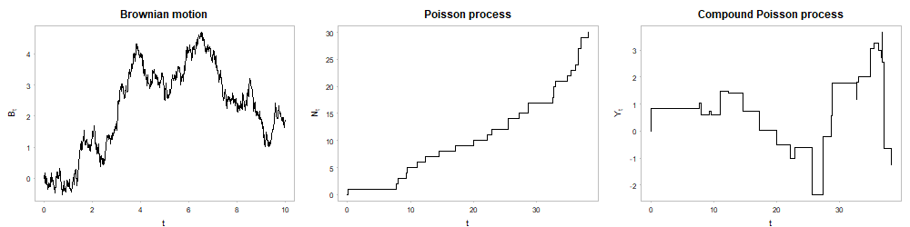
Fig. 15 Paths of a Brownian motion, a Poisson process and a compound Poisson process

Literature

App09(1,2)

David Applebaum. Lévy Processes and Stochastic Calculus. Volume 116 of Cambridge Studies in Advanced Mathematics. Cambridge University Press, Cambridge, 2. ed. edition, 2009.

Bas11

Richard F. Bass. Stochastic processes. Volume 33 of Cambridge series in statistical and probabilistic mathematics. Cambridge University Press, Cambridge, 1 edition, 2011.

Pro04

Philip E. Protter. Stochastic Integration and Differential Equations. Volume 21 of Stochastic Modelling and Applied Probability. Springer-Verlag, Berlin, 2. ed. edition, 2004.

Authors

Julian Wäsche

Contributors

Philipp Böttcher

---

1

More precisely, for any Lévy process, there exists a unique modification which is càdlàg \(\mathbb{P}\)-a.s. and which is also a Lévy process.