Parameter Identifiability for a Dynamical Model

Part of a series: Uncertainty Quantification for a Dynamical Model.

Follow reading here

The preceding article of this series discusses methods to estimate parameters of a system of ordinary differential equations (ODEs). In particular, maximum likelihood estimation and least squares estimation can be applied. Sometimes, however, it is not possible to identify parameter values unambiguously. The issue of parameter identifiability can mainly arise from two different sources. This article introduces these two notions of parameter identifiability. In order to detect non-identifiabilities, the concept of profile likelihoods is presented. Moreover, profile likelihoods allow to derive likelihood based confidence intervals to assess parameter uncertainty. If not stated otherwise, we adopt the model framework and the notation from the preceding article. To form a common ground, we nonetheless recall that we consider this system of ODEs

\[ \begin{align*} \frac{\mathrm{d} x(t)}{\mathrm{d} t}=f(t,x(t),\theta,u(t)),\quad x(0)=x_0(\theta)\in\mathbb{R}^N, \end{align*} \]

describing the dynamics of a state variable \(x\). The observation model, for obsvervables \(l=1,\dots,L\), is

\[ \begin{align*} y_l(t)=g_l(x(t),\theta)+\varepsilon_l(t,\theta),\quad\text{or}\quad y_l(t)=g_l(x(t),\theta)\cdot\varepsilon_l(t,\theta), \end{align*} \]

where the random variables \(\varepsilon_l\) represent measurement noise. The model parameters are summarized in the parameter vector \(\theta\in\Theta\) with parameter space \(\Theta\subset\mathbb{R}^{N_{\theta}}\). We assume that we have a data set \(y=(y_1,\dots,y_K)\in\mathbb{R}^{L\times K}\) containing measurements for each observable \(l\) measured at time points \(t_1,\dots,t_K>0\).

Definitions of Identifiability

In order to describe a real world phenomenon by an ODE model, unknown model parameters are usually estimated based on observed measurements. However, the accuracy of the parameter estimation is affected by the model’s parameterization as well as by the size and quality of the data set. These two sources basically distinguish the two main notions of parameter identifiability, structural and practical identifiability.

As the term may suggest, structural identifiability is related to the underlying model structure. For example, an inadequate model parameterization causes different parameter values to produce the same model output. In this case, a unique optimum value cannot be determined by parameter estimation [Raue et al., 2010]. In more formal terms, a parameter component \(\theta_i\) of \(\theta\), for \(i=1,\dots,N_{\theta}\), is then called structurally identifiable if its estimate \(\hat{\theta}_i\) is a unique maximum of the likelihood function \(\mathcal{L}(\theta)\) (or a unique minimum of the residual sum of squares \(\text{RSS}(\theta)\)) [Raue et al., 2009]. A model is structurally identifiable, if all model parameters are structurally identifiable. A more detailed discussion on structural identifiability is given in [Anstett-Collin et al., 2020] which also further distinguishes between local and global identifiability.

Even if a model is structurally identifiable, it may still be practically non-identifiable due to insufficient data (see plot in the middle of Fig. 25). The quality or quantity of experimental data may limit the information content to determine parameter values with finite confidence bounds. In light of that, a parameter component \(\theta_i\) is practically identifiable if the confidence interval of its estimate \(\hat{\theta}_i\) has finite size [Raue et al., 2009]. Again, if all model parameters are practically identifiable, a model is practically identifiable. Clearly, a parameter can be structurally identifiable but not practically identifiable, if the objective function has a unique optimum but the confidence interval of the estimate is of infinite length.

A more recent review on both structural and practial identifiability can be found in [Wieland et al., 2021]. In the next section, we introduce a likelihood-based approach to assess both structural and practical identifiability.

Profile Likelihoods

Confidence intervals for parameter estimates are usually constructed using the Fisher information. This approach is especially convenient for linear models. For more complex ODE models, profile likelihoods have been established to evaluate the shape of the log-likelihood function.

The profile likelihood of a parameter component \(\theta_i\), for \(i=1,\dots,N_{\theta}\), is defined by

\[ \begin{align*} \text{PL}_i(p)=\max_{\{\theta\in\Theta|\theta_i=p\}}l(\theta), \end{align*} \]

where \(l\) is the log-likelihood function of \(\theta\) [Raue et al., 2009]. By keeping fixed the component \(\theta_i=p\) and re-optimizing all other components \(j\neq i\), the profile likelihood \(PL_i(p)\) explores the parameter space for component \(j\). Thus, possible flatness of the likelihood can be detected by considering all components \(i=1,\dots,N_{\theta}\). In many cases, computing profiles can be challenging because multiple re-optimizations might become computationally costly.

Profile likelihoods allow to derive confidence intervals in order to assess the uncertainty of parameter estimates \(\hat{\theta}\) and to inspect identifiability. For \(\alpha\in(0,1)\), we denote by \(\Delta_{\alpha}(\chi_1^2)\) the \(\alpha\)-quantile of the chi-squared distribution with \(1\) degree of freedom. An asymptotic confidence interval for \(\theta_i\) at level \(\alpha\) is then given by [Kreutz et al., 2013]

\[ \begin{align*} CI_{\alpha}(\theta_i|y)=\left\{p\left|-2\cdot \text{PL}_i(p)\le -2\cdot l(\hat{\theta})+\Delta_{\alpha}(\chi_1^2)\right.\right\}. \end{align*} \]

In Fig. 25, the confidence intervals for different components of \(\theta\) correspond to the values lying below the threshold depicted by the dashed line. Based on these confidence intervals, non-identifiabilities can be revealed. If the profile likelihood of a component exhibits a flat shape and has no unique maximum, a structural non-identifiability is present (see plot on the right-hand side of Fig. 25). If there is a unique maximum, but the profile does not exceed the statistical threshold in both directions of the optimum, the component is practically non-identifiable (see plot in the middle of Fig. 25).

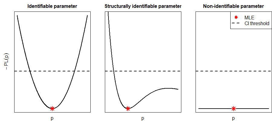
Fig. 25 The three cases of identifiability are depicted. The plot on the left-hand side represents the (negative) profile likelihood of a parameter that is both structurally and practically identifiable. The middle plot shows the profile of a parameter that is structurally identifiable, but not practically identifiable. The parameter of the right profile is neither structurally nor practically identifiable. The dashed line represents the threshold for confidence intervals.

The concept of identifiability and profile likelihoods for dynamical models can also be embedded in a Bayesian framework [Raue et al., 2013]. Moreover, these concepts are far from being limited to dynamical models [Murphy and van der Vaart, 2000, Walter and Pronzato, 1997].

To fit a model to data, “identifiability analysis is necessary to create good models” [Wieland et al., 2021]. This analysis assesses whether a model describes the data well and whether parameters can be accurately determined. This is crucial to be able to interpret statistical results and to draw meaningful conclusions about the underlying problem. However, in case of non-identifiabilities, the experimental setup might be improved to resolve these issues. The next article of this series covers the experimental design of a dynamical model in more detail.

References

ACDVM20

Floriane Anstett-Collin, Lilianne Denis-Vidal, and Gilles Millérioux. A priori identifiability: An overview on definitions and approaches. Annual Reviews in Control, 50:139–149, 2020.

KRKT13

Clemens Kreutz, Andreas Raue, Daniel Kaschek, and Jens Timmer. Profile likelihood in systems biology. FEBS Journal, 280:2564–2571, 2013.

MvdV00

Susan A. Murphy and Aad W. van der Vaart. On profile likelihood. Journal of the American Statistical Association, 95:449–465, 2000.

RBKT10

Andreas Raue, Verena Becker, Ursula Klingmüller, and Jens Timmer. Identifiability and observability analysis for experimental design in nonlinear dynamical models. Chaos, 2010.

RKM+09(1,2,3)

Andreas Raue, Clemens Kreutz, Thomas Maiwald, Julie Bachmann, Marcel Schilling, Ursula Klingmüller, and Jens Timmer. Structural and practical identifiability analysis of partially observed dynamical models by exploiting the profile likelihood. Bioinformatics, 25:1923–1929, 2009.

RKTT13

Andreas Raue, Clemens Kreutz, Fabian J. Theis, and Jens Timmer. Joining forces of Bayesian and frequentist methodology: A study for inference in the presence of non-identifiability. Philosophical Transactions of the Royal Society A: Mathematical, Physical and Engineering Sciences, 371:1–10, 2013.

WP97

Eric Walter and Luc Pronzato. Identification of Parametric Models from Experimental Data. Springer, 1997.

WHR+21(1,2)

Franz G. Wieland, Adrian L. Hauber, Marcus Rosenblatt, Christian Tönsing, and Jens Timmer. On structural and practical identifiability. Current Opinion in Systems Biology, 25:60–69, 2021.

Authors

Julian Wäsche

Contributors

Nabir Mamnun