Parameter Estimation for a Dynamical Model

Part of a series: Uncertainty Quantification for a Dynamical Model.

Follow reading here

In real-world applications, one of the main goals of statistical inference is to fit a model to data. If the object of interest is a parametric model, unknown parameter values are statistically inferred. This article focuses on parameter estimation of a parameterized system of ordinary differential equations (ODEs). For that matter, in line with frequentist statistics, model parameters are unknown but constant quantities. A Bayesian approach, where parameters are random variables with an underlying distribution, is, for example, applied in [Hasenauer, 2013]. It allows to incorporate prior knowledge about parameters that is updated with the information provided by measurements.

This article depicts methods to estimate the parameters of the reaction rate equation (RRE) from the preceding article. Even though RREs represent a particular type of ODEs, we study parameter estimation for a broader model framework [Kreutz and Timmer, 2009]. In the following, we therefore consider ODE models of the form

(5)\[ \begin{align} \frac{\mathrm{d} x(t)}{\mathrm{d} t}=f(t,x(t),\theta_x,u(t)),\quad x(0)=x_0(\theta_x)\in\mathbb{R}^N, \end{align} \]

where the dynamics of the state variable \(x\) are characterized by an \(\mathbb{R}^N\)-valued function \(f\). Typically, it is assumed that \(f\) is continuous in \(t\) and Lipschitz-continuous in \(x\) such that Equation (5) admits a unique solution [Adkins and Davidson, 2012]. The parameter vector \(\theta_x\in\mathbb{R}^{N_{\theta_x}}\) comprises the parameters of the state dynamics. External perturbations of the system are incorporated by an input function \(u(t)\) which can be time-dependent. For example, in a medical context, the function \(u(t)\) might represent stimulation by drug or hormone treatments or the regulation of genes [Kreutz and Timmer, 2009].

Observation Model

In real experiments, it is often infeasible to measure all state variables of \(x\) described by Equation (5) explicitly. Instead, only some of them or transformations are observed. These quantities are frequently called the observables of the system. Let us assume that there are \(l=1,\dots,L\) observables. The \(l\)-th observable is then defined as

\[ \begin{align*} i_l(t)=g_l(x(t),\theta_o), \end{align*} \]

where the \(\mathbb{R}\)-valued functions \(g_l\) link the system states to the observed quantities at time \(t\). If, for example, only parts of \(x(t)\) or a relative frequency are observed, then the functions \(g_l\) define projections on components of \(x(t)\) or a ratio, respectively. The observational function \(g\) might contain additional parameters denoted by \(\theta_o\in\mathbb{R}^{N_{\theta_o}}\).

Observed quantities are rarely measured exactly. Usually, measurements are subject to measurement error. Common error models involve additive or multiplicative noise [Kreutz et al., 2007]. Observations including one of this error types can then be written as

(6)\[ \begin{align} y_l(t)=g_l(x(t),\theta_o)+\varepsilon_l(t,\theta_{\varepsilon})\quad\text{or}\quad y_l(t)=g_l(x(t),\theta_o)\cdot\varepsilon_l(t,\theta_{\varepsilon}), \end{align} \]

respectively, where the \(\varepsilon_l\)’s are independent realizations of error distributions that need to be specified. The random variables \(\varepsilon_l\) might themselves depend on time \(t\) and on a parameter \(\theta_{\varepsilon}\in\mathbb{R}^{N_{\theta_{\varepsilon}}}\). If the error types are additive or multiplicative, a common choice for the error distribution is a normal distribution or a log-normal distribution, respectively.

Example

For our running example of a reaction system, we derived in the preceding article the RRE

\[\begin{split} \begin{align*} \mathrm{d} x_1(t)&=\left(c_1-c_2x_1(t)\right)\mathrm{d} t, \quad x_1(t_0)=x_1(0),\\ \mathrm{d} x_2(t)&=\left(c_2x_1(t)-c_3x_2(t)\right)\mathrm{d} t, \quad x_2(t_0)=x_2(0). \end{align*} \end{split}\]

We assume that only the relative amount of variable \(x_1\) can be measured directly. We further assume that observations are subject to additive and normally distributed measurement error. The observation model can thus be written as

\[ \begin{align*} y(t)=\frac{x_1(t)}{x_1(t)+x_2(t)}+\varepsilon,\quad t>0, \end{align*} \]

with \(\varepsilon\sim\mathcal{N}(0,\sigma^2),~\sigma>0\). The corresponding curve and simulated observations are depicted in Fig. 24.

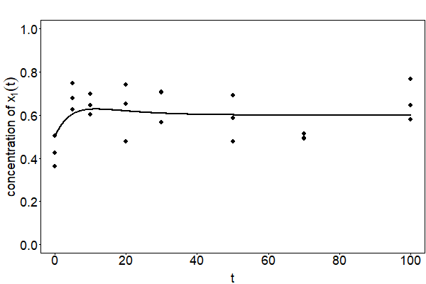
Fig. 24 The curve of the observation model with \(c_1=20,~c_2=0.1,~c_3=0.15,~x_1(0)=100\) and \(x_2(0)=100\) is depicted. The points represent observations that are simulated with \(\sigma=0.1\).

Before we deal with parameter estimation in the next section, we combine all model parameters into one parameter vector \(\theta=(\theta_x,\theta_o,\theta_{\varepsilon})\in\Theta\), where \(\Theta\subset\mathbb{R}^{N_{\theta}}\) denotes the parameter space with \(N_{\theta}=N_{\theta_x}+N_{\theta_o}+N_{\theta_{\varepsilon}}\).

Parameter Estimation

Based on the assumption that real data are overlaid with measurement noise, maximum likelihood estimation can be applied to estimate model parameters. Let \(y=(y_1,\dots,y_K)\in\mathbb{R}^{L\times K}\) be a data set containing measurements for each observable \(l=1,\dots,L\) measured at time points \(t_1,\dots,t_K>0\). The corresponding likelihood function is given by

\[ \begin{align*} \mathcal{L}(\theta)=\prod_{k=1}^K\prod_{l=1}^Lp_l(y_{k,l}|\theta), \end{align*} \]

where the function \(p_l\) denotes the probability distribution of the independently distributed measurements of the \(l\)-th observable. Taking the logarithm yields the log-likelihood function

\[ \begin{align*} l(\theta)=\ln\mathcal{L}(\theta). \end{align*} \]

The maximum likelihood estimator (MLE) is then defined by

(7)\[ \begin{align} \hat{\theta}=\underset{\theta\in\Theta}{\arg\max}~\mathcal{L}(\theta) =\underset{\theta\in\Theta}{\arg\max}~l(\theta). \end{align} \]

If the measurement errors are additive and normally distributed in (6), i.e. \(\varepsilon_{l}\sim\mathcal{N}(0,\sigma_{l}^2)\), with known standard deviations \(\sigma_{l}>0\), the MLE from Equation (7) coincides with the least squares estimator that minimizes the residual sum of squares

\[ \begin{align*} \text{RSS}(\theta)=\sum_{k=1}^K\sum_{l=1}^L\left(\frac{y_{k,l}-g_l(x(t_k),\theta)}{\sigma_{l}}\right)^2, \end{align*} \]

a measure for the squared differences of measurements and the observation model.

Maximum likelihood estimation and least squares estimation are two of the fundamental parameter estimation methods. However, depending on the problem at hand, several problems can arise with regard to parameter estimation. More advanced methods are reviewed in [Loskot et al., 2019] that aim to solve these problems. One of these problems is the issue of parameter identifiability that may hamper parameter estimation. It is not guaranteed that the likelihood function has a unique maximum such that parameter values might not be identified unambiguously. The next article of this series discusses this issue in more detail.

References

AD12

William A. Adkins and Mark G. Davidson. Ordinary Differential Equations. Springer, 2012.

Has13

Jan Hasenauer. Modeling and parameter estimation for heterogeneous cell populations. University of Stuttgart (PhD Thesis), 2013.

KRM+07

Clemens Kreutz, Maria M.Bartolome Rodriguez, Thomas Maiwald, Maximilian Seidl, Hubert E. Blum, Leonhard Mohr, and Jens Timmer. An error model for protein quantification. Bioinformatics, 23:2747–2753, 2007.

KT09(1,2)

Clemens Kreutz and Jens Timmer. Systems biology: Experimental design. FEBS Journal, 276:923–942, 2009.

LAM19

Pavel Loskot, Komlan Atitey, and Lyudmila Mihaylova. Comprehensive review of models and methods for inferences in bio-chemical reaction networks. Frontiers in Genetics, 2019.

Authors

Julian Wäsche

Contributors

Kuan-Yu Ke