The Mathematical Perspective on Mapping Uncertainty in scRNA Experiments#
Part of a series: Uncertainty in scRNA experiments.
Follow reading here
Introduction#
Sequencing biological samples leads to short nucleotide sequences which are called raw reads (see Fig. 65). Of primary interest, however, are not these sequences themselves, but their genomic origin. Hence, additional steps, which are often summarized as preprocessing, are required before further analyses like clustering or extracting principle components can be performed. One part of preprocessing is the mapping of raw reads to their most plausible genomic origin. This article deals with a mathematical representation of this particular mapping-step and how uncertainty affects its performance. For the sake of simplicity, this article focuses mostly on the unique mapping approach. The term has been coined by [Mortazavi et al., 2008].
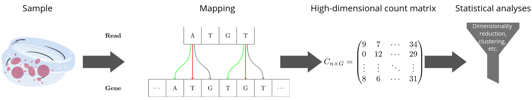
Fig. 65 From a biological sample (here blood cells) to the observed count data which is to be analyzed statistically.#
The Mathematical Framework#
Each gene \(g\in \{1,\dots,G\}\) consists of a fixed number of nucleotides, \(N_g \in \mathbb{N}\), and each such nucleotide, in turn, can be adenine (A), thymine (T), guanine (G) or cytosine (C). All possible gene sequences with length \(N\) can hence be represented by the cartesian product \(\Omega_{N} = \{A,C,G,T\}^{N}\). If we include spaces (S) for shorter genes and denote \(N_{\bar G}:=max_{g=1,\dots,G}\{N_g\}\), we can easily generalize this to become the set of all possible genes. The number of possible sequences grows exponentially with respect to their lengths because \(|\Omega_{N_{\bar G}}|=5^{N_{\bar G}}\). Nevertheless, this set remains finite for any fixed \(N_{\bar G}\). Moreover, we can oftentimes narrow it down even further by including prior knowledge. For instance, the human genome has been studied exhaustively and only a very small fraction (i.e. ca. \(21000\)) of the roughly \(5^{20000}\) possibible sequences are actual genes.
The costs for a genomic sequence to be extracted from a sample are closely related to its length. Hence sequencing whole gene sequences is almost impossible. Instead, we collect \(R\in \mathbb{N}\) much shorter (potentially erroneous) pieces from these genes: the raw reads. Fortunately, the mathematical set-up is almost equivalent for reads. The only difference is that their maximal length, \(N_{\bar R}\) is a lot smaller than \(N_{\bar G}\) which also reduces the size of the read space, i.e. \(|\Omega_{\bar R}| < |\Omega_{\bar G}|\).
Finally, the true mapping of any read to its genomic origin is from a mathematical perspective just a function \(m:\Omega_{\bar R} \to\{1,...G\}\). In plain words, every read emerged from one particular gene and thus a certain rule or algorithm should exist to map both. The challenge is to find a suited approximation of \(m\).
In practice, it is not always possible to determine exactly one genomic origin for every read. So instead of pointing towards just one gene, most modern mapping approaches derive first a set of \(k\) possible origins, i.e. \(\hat m:\Omega_{\bar R} \to\{1,...G\}^k\), and based on that a probability distribution over all possible genomic origins, i.e. \(q:\{1,...G\}^k \to [0,1]^G\). Please note the different notation between a mapping approach, denoted by \(\hat m\), and the true genomic origin \(m\). The second step is often called quantification and will not be considered further in this article.
Implications of Unique Mapping#
The simplest, but still yet used mapping procedure is unique mapping. Here, only perfect matches of a read to exactly one particular gene are counted. Hence a uniquely mapped read is a subsequence of exactly one gene at exactly one position. It is of great importance for microbiologists to know if and under what conditions this approach leads to reliable results. Potential questions include how long reads shall be to be mapped with a certain probability, and how the organism of interest affects this accuracy (e. g. via number of genes and their lengths). Throughout this section we will investigate the two driving factors of unique mapping:
Has the read been sequenced correctly?
What is the ratio between read and reference lengths?
The implication of the first question is straightforward. A correctly sequenced read will always fit perfectly to the true genomic position. However, this match is not necessarily unique. Just by chance, the exact same sequence of nucleotides of the read could be apparent in multiple genes and multiple locations. Imagine, for instance how much easier it is for you to find words containing “ing” than “reseeing”. In addition, some nucleotide sequences may occur more often in genes than others. Likewise, many more English words include the string “ing” than “xyy”. This behavious is often referred to as non-uniform base distributions and some algorithms account for it using empirical nucleotide (or \(k\)-mer) frequencies. However, we will neglect base distributions for now in order to derive a first simple mathematical model. Given uniform base distributions, the probability of matching a correct read to one additional position of the true gene of origin is determined by its length and the size of the gene. Denoting the set of correctly sequenced reads by \(C \subset \{1,\dots,R\}\) we can approximate1 this chance by
The formula above describes the probability of finding all \(N_r\) bases in a gene \(g\) at exactly \(1\) (not counting the true origin here) out of the potential \(N_g-N_r\) positions2. Please note that we focused on correctly sequenced reads only. Here, the true origin will always be found, i.e. \(m(X_r) \in \hat m(X_r) \Rightarrow |\hat m(X_r)| \geq 1\) since \(X_r \subset X_g \iff m(X_r)=g\). This is why the probability formula above solely depends on the additional match. Please note that non-uniform base distributions would lead to a more complicated read probability than \((1/5)^{N_r}\).
What happens when we want to consider all genes? So instead of approximating the chance for an additional match in one particular gene, we want to know the probability of a second match anywhere in the genome. Unfortunately, we cannot simply sum up the probabilities from the formula (16) over all genes because this would give us the chance of finding exactly one additional match in every gene. Instead, we have to take all combinations of matches into account that yield one (or more generall \(p\)) overall additional mapping. This can be defined by the set \(K(p):= \{k\in\mathrm{N}_0^G|\sum_g k_g = p\}\). For instance, \(K(1)\) is the set of all \(G\)-dimensional unit vectors and hence provides us with all combinations that yield exactly one additional match (regardless of the particular gene). Equipped with these quantities we can generalize the probability of multiple matches to
In plain words, the formula above adds up the chances for all combinations \(K(p)\) that yield \(p\) additional matches. This is done via the gene-specific binomial probabilities. Please note the implicit assumption that all genes are independent and thus their joint distribution can be derived simply as a product.
Example: Minimal Read Lengths for Unique Mapping to Homo Sapiens Genome#
The R-Script below shows how to access and study a reference sequence. For this example, the transcriptome of Homo Sapiens (containing roughly 11700 transcripts) has been downloaded from Ensembl. Readers, who do not know about the difference between genome and transcriptome, should think about them as equal. For the sake of accuracy, we will still refer to the reference as transcriptome though.
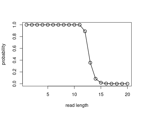
For a first investigation, we want to neglect the actual nucleotide sequences and use only its length. For this, we can treat all reference sequences as one large transcript with \(N_{total}=\sum_g N_g=538785055\) nucelotides. With this we can approximate the probability of at least one additional match by \(\sum_{p\in \mathbb{N}} \eta(p) \approx 1- \binom{N_{total}-N_r+1}{0} \left( \frac{1}{5} \right) ^{N_r}\). The following figure shows that longer reads indeed reduce this probability.
# Prerequisites:
# 1. Install BiocManager and with this, the packages below.
# 2. Download the Homo Sapiens reference sequence e.g. from ensembl.org/
library(polyester)
library(Biostrings)

path_to_genome = "~/ensemble_HSapiens_chrom5.txt"
fasta = readDNAStringSet(path_to_genome)
Ng = width(fasta)
hist(Ng)
N_total = sum(Ng)
additional_match = function(Ng, Nr, k){
  1-dbinom(0, size = Ng-Nr+1, prob = (1/5)^Nr)
}
probs = additional_match(N_total, 1:20, 1)
plot(1:20, probs, lwd=1.5, cex=1.5, type="o", xlab="read length", ylab="probability")
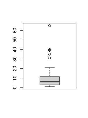
Our previous approach makes several restrictive assumptions which probably do not hold in practice. For instance, we assumed that all reads and genes are identically distributed in the sense that only their lengths matters. The next code snippet draws \(100\) reads of length \(20\) as random subsequences from the reference and then searches for candidates without mismatches in the reference. According to the previous graphic, we should expext almost no reads with multiple mappings. The boxplot below, however, draws a different picture. Apparently, reads and genes are not random sequences. In fact multiple matches are much more likely and only roughly \(20\%\) have been mapped uniquely. Some reads even fit to over \(100\) positions. It would be interesting to study this issue for more reads, but our naive mapping approach is computationally too intensive.
s <- sample(length(fasta), 100)
N_g = as.vector(sapply(fasta, length))
starts = sapply(N_g-30, FUN= function(x) sample(1:x,1))
reads = subseq(x=fasta[s], start=starts[s], width=20)
reads[1] # See how a nucleotide sequence as S4 object looks like
# The following code takes some time!
matches = sapply(reads, FUN = function(x){
  v1 = vmatchPattern(as.character(x), fasta)
  matches = length(unlist(extractAt(fasta, v1)))
  return(matches)
})
boxplot(matches[matches<100])
summary(matches)
If the read is erroneous, opposite conclusions can be drawn. We will definetly not map the read to its true origin, but we may find other matches by chance again. In fact we can use the derivations from before because \(\Pr( |\hat m(X_r)|=p|r \notin C) \approx \Pr( |\hat m(X_r)|=p+1|r \in C) =\eta(p)\). Hence the overall unique mapping likelihood may be described using the law of total probability:
Analogously, one could derive the counter-probability of a multiread, i.e. a read with at least one additional match which would be discarded in unique mapping. Hence, this formula could be used to answer the initial questions of this chapter if we knew all the quantities. But of course the a priori probability of a read to be correct is unknown. If we knew this, we would have discarded all erroneous reads in the first place.
Let us assume for a moment that we have chosen our reads fairly long and the number of incorrect reads is relatively small. In that case, we could be rather sure to fit almost all correct reads uniquely and the incorrect reads would cause almost no harm to the estimation. Nonetheless, the results still rely on the mathematical assumptions made in the derivation above. Especially, highly similar genes and correlated errors undermine the reliability of unique mapping. The former issue leads to lots of multiple matches in several similar genes which would be discarded alltogether in unique mapping. The gene expression levels for these similar genes would hence be underestimated. Analogously, correlations between erroneous reads and gene-specific attributes may cause trouble. Imagine, for instance, higher sequencing errors for longer genes or regarding the adenine-base.
Tackling the Uncertainty#
One can look at the unknown error probability \(\Pr(C)\) from two angles.
How certain is the sequencer about the read’s quality?
Can I weight different matches with according to some additional information?
Many modern machines for scRNA sequencing provide quality scores alongside the raw reads. Strictly speakig, the sequencer measures the trust in the correctness of the sequenced nucleotides. One such measure is Phred’s score [Ewing et al., 1998] which essentially compares the signals of every sequenced nucleotide and assigns a quality value in \([4,60]\) using the following normalized error probability \(-10 \log_{10} \Pr(\text{base error})\). The last quantity takes into account the form and strength of signals (i. e. sequencing peaks) at every base. The higher the Phred’s score of a sequenced base, the more reliable is the nucleotide information. This score can be incorporated in mapping methods, for instance, when replacing the number of allowed mismatches by a maximum value for the sum of their Phred’s scores.
Of course, more sophisticated and therefore more accurate mapping methods have been developed during the last decades. Many of them include an iterative scheme which alternates between mapping and quantifying gene-specific parameters. This is done to account for the gene-specific information in the priorization of candidates. Take, for instance, the so-called rescue method [Mortazavi et al., 2008] which allocates non-unique mappable reads based on their unique counterparts. Conceptually, this equals one iteration from the previously mentioned alternating schemes. At first, only unique reads are considered to calculate gene expression levels \(\hat \theta \in [0,1]^G\) (i. e. the relative frequencies of unique reads from every gene). The non-unique reads are then allocated based on the following weighted average: \(\frac{\theta_g}{\sum_{g' \in m(X_r)}\theta_{g'}}\). It makes intuitive sense that rescuing (or recycling) the multiple mapped reads increases the accuracy. Describing the mathematic details behind it, however, becomes more difficult.
References#
- EHWG98
Brent Ewing, LaDeana Hillier, Michael C Wendl, and Phil Green. Base-calling of automated sequencer traces usingphred. i. accuracy assessment. Genome research, 8(3):175–185, 1998.
- MWM+08(1,2)
Ali Mortazavi, Brian A. Williams, Kenneth McCue, Lorian Schaeffer, and Barbara Wold. Mapping and quantifying mammalian transcriptomes by rna-seq. Nature Methods, 5:621–628, 2008. doi:10.1038/nmeth.1226.
Contributors#
Julian Wäsche
- 1
Because the assumption that a gene is a random sequence of nucleotides is unlikely to be true in practice.
- 2
In fact, we have \(N_g-N_r+1\) positions, but the true one is of no interest for the additional match. The good news are that for large \(N_g\), which is the case for genetic sequences, the difference diminishes. For the sake of correctness, we will still use approximative equalities in this article whenever this scenario is neglected.