UQ in scRNA-Seq Experiments#
This article is part of a series: Uncertainty quantification in scRNA-Seq experiments. The following aspects are covered
Introduction#
Scientists today are still puzzled by many diseases that are related to changes on the level of gene expressions, such as cancer. In plain words, such a disease affects a cell’s ability to replicate or create potentially important proteins. Studying, for instance, blood or tissue samples can help to understand the underlying microbiological mechanism, the progression of a disease itself and finally to deduce appropriate treatments. Therefore, it is necessary to quantify gene expressions in a sample, and distinguish healthy from infected cells adequately. However, one cannot observe and count these molecules directly. Instead, several intermediary steps are necessary which lead to millions of duplicated and much shorter RNA sequences. This article discusses the impact of the RNA-Seq [Nagalakshmi et al., 2008] set-up on the estimation accuracy of gene expressions as well as the various sources of uncertainty that are involved.
Single-cell RNA-Seq#
The term RNA-Seq refers to a variety of sequencing protocols with the goal to obtain nucleotide sequences from a sample. These nucleotide sequences are then statistically analyzed to reconstruct a genome, count abundances or find latent structures wihin a sample. The following figure highlights the main steps in an RNA-Seq sequencing procedure. Since whole mRNA molecules are simply too long for sequencing, they are cut into smaller fragments. The subsequent amplification step doubles the sample size iteratively by cloning each template. Afterwards the sample contains bulks of equivalent fragments which are visualized in parallel by a high-throughput sequencer. The final observable measurements are millions of short nucleotide sequences, so-called reads, which are assumed to appear proportional to the initial RNA sample and mapped back to the reference genome. [Conesa et al., 2016] review good practices in the field of RNA-Seq data analysis.
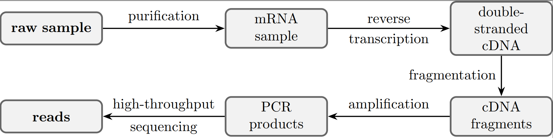
Fig. 63 Schematic representation of typical steps from single cell RNA-Seq protocols.#
Recent technological advances enabled microbiologists to apply such protocols repetitively even on the level of single cells. Hence, cell heterogeneity can be captured, outlier cells detected and distributional forms derived in order to tell groups of cells apart. The following figure sketches how gene expression levels may differ for groups compared to outliers.
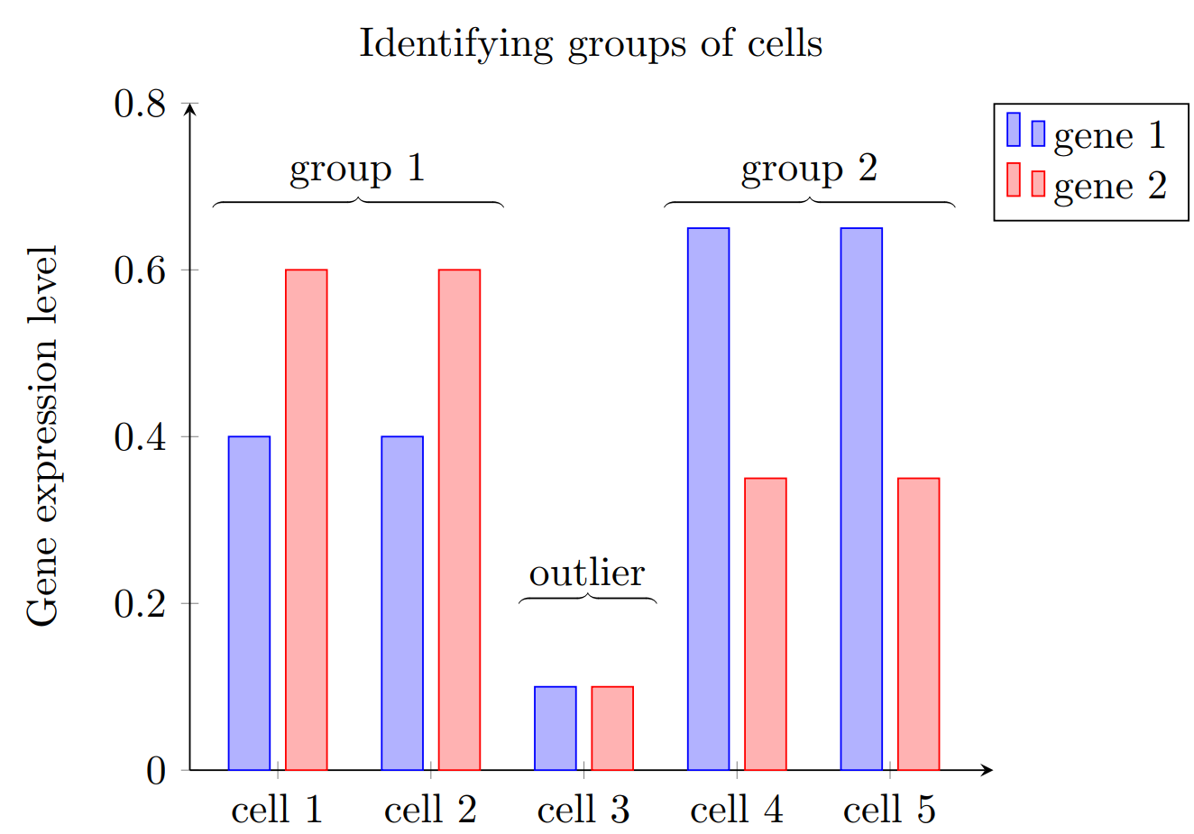
Fig. 64 Clustering cells into groups based on their gene expressions.#
Sources of Uncertainty#
It is unsurprising that a complex process such as the amount of mapped reads includes various sources of uncertainty. They can be classified into the following groups:
Biological uncertainty
Experimental uncertainty
Modelling uncertainty
Biological uncertainty refers to the in vivo number of expressed molecules within each cell in an organism that is inherently stochastic. This may be seen as the in-cell equivalent of demographic noise. The only difference is that we are not interested in the composition of a population of cells, but the composition of gene expressions for one particular cell. Due to such natural uncertainty, one cannot predict the number of mRNA molecules per gene perfectly, but must account for this cell heterogeneity. Only understanding and modelling the variability correctly allows for accurate uncertainty quantification.
Furthermore, the whole RNA sequencing procedure greatly affects the estimation of expressions. For instance, how a sample reacts to each of the sequencing steps might depend on external factors like temperature, waiting times, and pressure. Also the polymerase chain reaction can produce erroneous sequences which are then again used as erroneous templates in later amplification cycles. Even if a read is sequenced correctly, it might fit to multiple genomic positions. A preprocessing step called mapping tackles this particular problem. This article sheds light on the mathematical perspective of selected mapping approaches. Overall, the outcome might vary even with identical raw samples as input! The amount of uncertainty added by these kind of experimental set-ups is referred to as experimental or measurement uncertainty.
Given a sample, the statistical analysis of gene expression levels is oftentimes based on data-related and distributional assumptions, e.g. statistical independence and an identical density distribution for all individuals (“iid”) or a specific parametric density distribution. The term model uncertainty summarizes this lack of knowledge regarding the form of the data generating process. Especially in scRNA-Seq, it remains unknown, whether the distributional form for mapped reads is equivalent or at least comparable to that of the mRNA molecules.
Dealing with Uncertainty in scRNA-Seq#
The data for the statistical analysis are the number of reads mapped to their genomic origin \(g\) for \(I\) single cells denoted by \(\{X_{i,g}\}_{g\leq G, i \leq I}\). Without normalization this data is a count matrix of absolute abundances that represents \(I\) (hopefully independent) realizations from a gene-specific \(G\)-dimensional count process. The goal is to identify and analyze the uncertainty from the various sources by an appropriate probabilistic model. Due to the discussed cell heterogeneity, the parameter for the gene expression level \(\theta\in [0,1]^G\) is likely to vary and hence has its own distribution e.g. \(\theta|\alpha \sim \text{Dir}(\alpha)\). The Dirichlet distribution is just one out of many possible distributions which generalizes the Beta distribution to \(G\)-dimensional probability vectors. Moreover, many samples contain thousands of potentially highly correlated genes. The Hamiltonian Monte Carlo (HMC) method implemented as No-U-Turn sampler from [Hoffman and Gelman, 2014] provides an efficient algorithm for the estimation of such high-dimensional problems. This Markov Chain Monte Carlo (MCMC) uses Hamilton dynamics expressed as differential equations to mimic the movement of a marble on a surface. A good description can be found in [Neal, 2011]. Since the surface is related to the target distribution, HMC accounts for its structure and hence generates more adequate proposals to prolongate the Markov chain. These proposals are accepted more often which finally shortens the time to convergence of the Markov chain. Additionally, knowledge from publicly available data can be included in the model prior.
References#
- CMT+16
Ana Conesa, Pedro Madrigal, Sonia Tarazona, David Gomez-Cabrero, Alejandra Cervera, Andrew McPherson, Michał Wojciech Szcześniak, Daniel J Gaffney, Laura L Elo, Xuegong Zhang, and others. A survey of best practices for RNA-seq data analysis. Genome Biology, 17(1):1–19, 2016.
- HG14
Matthew D. Hoffman and Andrew Gelman. The no-U-turn sampler: Adaptively setting path lengths in Hamiltonian Monte Carlo. Journal of Machine Learning Research, 15:1593–1623, 2014. URL: https://www.jmlr.org/papers/volume15/hoffman14a/hoffman14a.pdf.
- NWW+08
Ugrappa Nagalakshmi, Zhong Wang, Karl Waern, Chong Shou, Debasish Raha, Mark Gerstein, and Michael Snyder. The transcriptional landscape of the yeast genome defined by RNA sequencing. Science, 320(5881):1344–1349, 2008.
- Nea11
Radford M. Neal. MCMC using Hamiltonian dynamics. Handbook of Markov Chain Monte Carlo, pages 113–162, 2011. doi:10.1201/b10905-6.
Contributors#
Sonja Germscheid