Hamiltonian Monte Carlo#
Introduction#
Hamiltonian Monte Carlo is an MCMC sampler and to be more precise, it is a special case of the Metropolis Hastings algorithm. This means Hamiltonian Monte Carlo is used to create samples which eventually will follow a certain target distribution \(F\). Hamiltonian Monte Carlo differs from the standard Metropolis Hastings algorithm in terms of the proposal mechanism. Hamiltonian dynamics are used in physics to describe the path of an object on a surface. A helpful illustration is to think about placing a marble in a bowl and randomly pushing it in some direction. After the initialization, the marble follows a system of physical equations which describe its path. This concept is adapted in Hamiltonian Monte Carlo by drawing new candidates based on the movement of a virtual marble that rolls on (means according to) our target distribution [Betancourt, 2017].
The Algorithm#
The parameters of interest are denoted as the position \(q_t \in \mathbb{R}^d\) of the marble. To fully describe the physical system, auxiliary momentum variables \(M \cdot v_t = p_t \in \mathbb{R}^d\) are required. The momentum, \(p_t\), of the marble is the product of its mass \(M\) and current velocity \(v_t\). The joint (or canonical) distribution of such a system in physics is described by \(\pi(q_t,p_t)= \frac{1}{Z} \exp(-H(q,p)/T)\). Here \(Z\) is used for normalization, \(T\) denotes the (normalized) temperature of the system and \(H\) is the energy in the current state (also referred to as Hamiltonian). In Hamiltonian Monte Carlo, the total energy is the sum of
potential energy, \(U(q_t)=-\log (\pi(q_t))\), held by the marble because of its relative position and
kinetic energy, \(K(p_t)=\frac{Mv_t^2}{2}=\frac{p_t^TM^{-1}p_t}{2}\), needed to accelerate the marble from \(0\) to \(v_t\).
This set-up ensures that Hamiltonian Monte Carlo samples from the target distribution \(\pi(q_t)\) and that the initial momenta can be drawn independently via \(p_i \sim N(0,m_i)\). Afterwards, the marble follows Hamilton’s equation:
Please note that the derivative of \(U\) requires the parameters to be continuous and does not always have a trivial form. Hence, this approach is often computationally more costly than classical Metropolis Hastings. Moreover, the differential equation (DE) systems are not solvable in general and a discretization with respect to the time \(t\) is needed anyway in order to create a Markov chain.
In practice, the leapfrog method is used to approximate the DEs after every \(\epsilon\) time points for a total of \(L\) steps. The leapfrog scheme is similar to the Euler approximation, but preserves the volume perfectly since it updates the state parameters asynchronously. After the initial momentum was drawn, half a step is made for the momentum variable. Based on this, the position and momentum vectors are updated iteratively by making full steps of length \(\epsilon\). In the end, another half step is performed for the momentum. The whole procedure may be described by the following sketch:
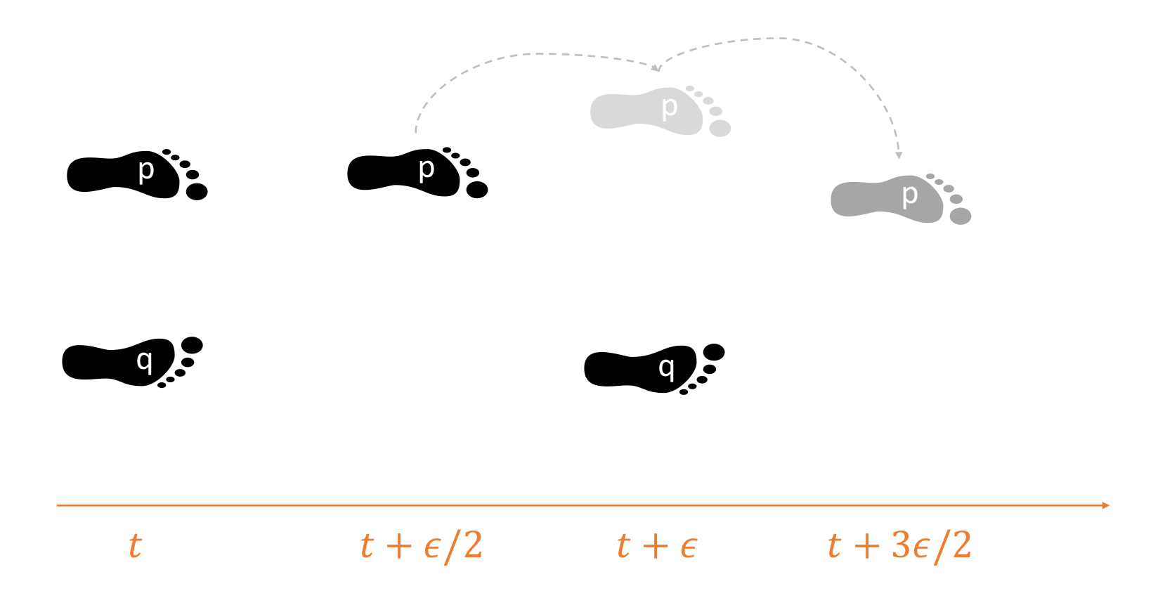
Fig. 28 Graphical representation of asynchronous Euler steps to preserve volume.#
Examples#
A simple example consists of a one-dimensional parameter \(m=d=1 \quad \Rightarrow \quad q(t),p(t) \in \mathbb{R}\). In addition, we fix the potential energy to be the parabola \(U(q) = \frac{q^2}{2}\) because Hamiltonian Monte Carlo then samples from a standard normal distribution. Due to the particular mass, the kinetic energy takes exactly the same form, i.e. \(K(p)=\frac{p^2}{2}\) and hence the total energy is the circle equation \(H(q,p) = \frac{q^2+p^2}{2}\). At each state \((q_t,p_t)\) the marble has a certain energy \(H\) and moves along the parabola by altering the state parameters on the circle. Luckily, the DEs can be solved analytically in this case and lead the following equations for future positions and momenta:
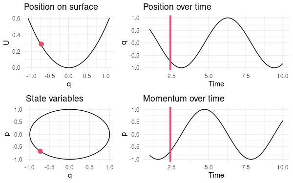
Fig. 29 Single frame from a continuous R shiny simulation to emphasize the relation between position and momentum in Hamiltonian Monte Carlo.#
Applications#
For the application of Hamiltonian Monte Carlo, the leapfrog scheme must be programmed. A minimalistic example in the programming language R is available in [Neal, 2011]. Although this works fine for smaller problems and grasping the steps within the algorithm, this code is not scalable without further adaptions.
A great alternative provides the platform STAN which uses a run-time optimized and CPU-parallelized C++ enginge for calculations and offers an interface to most of the popular computer softwares (e.g. python, R, Julia) for the user.
Ambiguities and Field-specific Meaning#
It is indeed noteworthy that Hamiltonian Monte Carlo compromises between continuous-time DEs and classical Markov chains. The concept of Markov chains can also be extended to continuous time and is usually based on generators which also require a solution of the assumed DEs. Depending on the curvature of the target function, the discretization carried out in Hamiltonian Monte Carlo can lead to inefficiency (\(\epsilon\) too small) in some regions and divergent transitions (\(\epsilon\) too large and hence \(H\) not constant) in others.
References#
- Bet17
Michael Betancourt. A Conceptual Introduction to Hamiltonian Monte Carlo. arXiv e-prints, 1 2017. URL: http://arxiv.org/abs/1701.02434.
- HG14
Matthew D. Hoffman and Andrew Gelman. The no-U-turn sampler: Adaptively setting path lengths in Hamiltonian Monte Carlo. Journal of Machine Learning Research, 15:1593–1623, 2014. URL: https://www.jmlr.org/papers/volume15/hoffman14a/hoffman14a.pdf.
- Nea11
Radford M. Neal. MCMC using Hamiltonian dynamics. Handbook of Markov Chain Monte Carlo, pages 113–162, 2011. doi:10.1201/b10905-6.
Contributors#
Houda Yaqine, Hendrik Paasche