Stochastic Differential Equations

Part of a series: Stochastic fundamentals.

Follow reading here

A stochastic differential equation (SDE) is a mathematical description for a process with stochastic fluctuations, i.e., some form of noise of fast oscillations. As the name suggests, it is a mathematical model constructed using differential forms, commonly comprising two elements: a deterministic motion and a stochastic fluctuation. A stochastic differential equation is very similar to an ordinary differential equation, to which an element of noise, e.g. a Brownian noise, is added. This nevertheless requires a thorough reevaluation of several mathematical tools in order to make sense. For example, a new form of integration is usually required to handle the stochastic fluctuations.

A typical stochastic differential equation for a random variable \(X_t\) is time \(t\) takes the form

\[ d X_t = f(X_t,t)d t + g(X_t,t) dB_t, \]

but this should be view as a representation of the integral form

\[ X_{t+s} - X_t = \int_t^{t+s} f(X_u,u)d u + \int_t^{t+s} g(X_u,u) dB_u, \]

where \(B_t\) is a Wiener process or Brownian motion. Here one distinguishes clearly the integral \(\int_t^{t+s}\dots d u\) as a Lebesgue integral and an integral form suitable for the stochastic noise \(B_t\) called the Itô integral, named after its inventor Kiyoshi Itô.

From an application point-of-view, one usually has a recording of a stochastic process, which can be single dimensional or in \(N\) dimensions. These data, or timeseries, have a distinct property of having noise around a deterministic motion or trend. An SDE allow one to describe both the deterministic motion and the fluctuations around these.

From ODEs to SDEs

Consider the following ordinary differential equation:

\[\begin{split} \begin{cases} \frac{dX(t)}{dt}&=f(X(t)), \ t>0\\ X(0)&= X_0 \end{cases}\ \ \ (1) \end{split}\]

Where \(f:\mathbb{R} \to \mathbb{R}\) is a smooth function. The solution to such equation is the function \(X:[0,\infty[\to \mathbb{R}\).

Often, it is hard to predict or understand certain aspects of the dynamics underlying real world applications (e.g. biological phenomena) and are thus represented by noise. Unfortunately ODEs cannot count for noisy components and thus need some extensions. To compensate the deficiency, stochastic differential equations (SDEs) were introduced.

SDEs are a natural extension of ODEs to account for that external noise, by adding a diffusion term to the equation. A formal way to express this is:

\[\begin{split} \begin{cases} \frac{dX(t)}{dt}&=f(X(t))+g(X(t))\xi(t),\ t>0\\ X(0)&=X_0 \end{cases}\ \ \ (2) \end{split}\]

where \(g:\mathbb{R} \to \mathbb{R}\) is called the diffusion term and it tells how the noise enters the system, the function \(f\) is called the drift function and it represents the nominal dynamics of the system, while \(\xi (.)\) is a white noise. The above equation turns out to be:

\[\begin{split} \begin{cases} dX(t)&=f(X(t))dt+g(X(t))dW(t),\ t>0\\ X(0)&=X_0 \end{cases}\ \ \ (3) \end{split}\]

where \(W(t)\) is a Brownian motion, which is an abstract version of a random walk, that is the increments are completely random and independent.

Depending on the functions \(f\) and \(g\), we can classify SDEs into two large groups, linear SDEs and non-linear SDEs. Furthermore we can also distinguish between scalar and vector-valued SDEs.

The Fokker–Planck equation

Fokker–Planck equation is a central equation in the description of stochastic processes from the point-of-view of their distributional properties. In some sense, when dealing with a stochastic process, there are two sides of a coin: on one hand an SDE details a particular realisation or evolution of a random variable \(X_t\) in time (or space), on the other hand, at each time \(t\) and point in space \(x\) one can attribute a certain probability of finding \(X_t\) at \(x\).

The Fokker–Planck equation is a partial differential equation for the conditional probability density function \(p(x,t|x',t')\) from a family of processes (1) given by

\[ \frac{\partial}{\partial t} p(x,t|x',t') = -\frac{\partial}{\partial x} f(x, t) p(x,t|x',t') + \frac{\partial^2}{\partial x^2}g(x,t) p(x,t|x',t'). \ \ \ (3*) \]

This equation is valid for continuous Markovian stochastic processes. A generalisation from discontinuous processes, i.e., including jumps, is possible via the Kramers–Moyal expansion. The conditional moments \(K_n(x,t,\Delta t)\) are given by

\[ K_n(x,t,\Delta t) = \int (y-x)^n p(y,t+\Delta t|y,t) dy \ \ \ (4*), \]

which in the limit of \(\Delta t\to 0\) results in the Kramers–Moyal coefficients

\[ D_n(x,t) = \frac{1}{n!}\lim_{\Delta t \to 0} \frac{1}{\Delta t}K_n(x,t,\Delta t) \ \ \ (5*) \]

which for the particular case of \(n=1\), \(D_1(x) = f(x)\), the drift function, and \(n=1\), \(D_3(x) = g(x)\) the diffusion function as given in (3). Conditional moments \(K_n(x,t,\Delta t)\) and Kramers–Moyal coefficients \(D_n(x,t)\) are not bound to only having order \(n=1\) and \(n=2\), but for a continuous stochastic process, these are the only two contributing terms

For more details on why a continuous stochastic process is fully represented by the two first moments, see Pawula’s theorem

The Kramers–Moyal expansion

Take a Markov process \(X_t\) that is described by a conditional probability density function \(p(x,t|x',t')\). The probability density function at time \(t+\tau\) is given by

\[ p(x,t+\tau) = \int p(x,t+\tau|x',t) p(x',t) dx', \]

where the integration over \(x'\) should encompass all possible values of \(x'\). Rewrite the conditional probability \(p(x,t+\tau|x',t)\) as

\[ p(x,t+\tau|x',t) = \int \delta(y-x) p(x',t) p(y,t+\tau|x',t) dy, \]

and expand the \(\delta\)-function as

\[ \delta(y-x) = \sum_{n=0}^\infty \frac{(y-x')^n}{n!} \left(-\frac{\partial}{\partial x'}\right)^n \delta(x'-x). \]

By substitution one obtains

\[ p(x,t+\tau|x',t) = \sum_{n=0}^\infty \frac{1}{n!} \left(\frac{\partial}{\partial x'}\right)^n \int (y-x')^n p(y,t+\tau|x',t)\delta(x'-x). \]

Here note that this is just the definition of the the conditional moments \(K_n(x,t,\Delta t)\) given in (4*), thus

\[ p(x,t+\tau|x',t) = \left[1+\sum_{n=1}^\infty \frac{1}{n!} \left(-\frac{\partial}{\partial x}\right)^n K_n(x,t,\tau) \right] \delta(x'-x). \]

Take the difference

\[ p(x,t+\tau) - p(x,t) = \frac{\partial p(x,t)}{\partial x} + \mathcal{O}(\tau^2) = \sum_{n=1}^\infty \frac{1}{n!} \left(-\frac{\partial}{\partial x}\right)^n \int K_n(y,t,\tau) \delta(y-x) p(y,t) \]

And subsequently divide by \(\tau\) and take the limit of \(\tau \to 0\)

\[ \frac{\partial p(x,t)}{\partial x} = \sum_{n=1}^\infty \frac{1}{n!} \left(-\frac{\partial}{\partial x}\right)^n D_n(x,t,) p(x,t) \]

Where one recovers the Kramers–Moyal coefficients \(D_n(x,t)\) as given by (5*).

If we truncate this expansion at order \(n=3\), keeping only the first and second-order terms, we recover the Fokker—Planck equation (3*).

Solutions to SDEs

Because white noise is nowhere differentiable, we cannot use the same theory for ODEs to solve SDEs. An alternative way would be to extend numerical approximation methods, such as Euler-Maruyama scheme or Milstein scheme to approximate the solutions of SDEs, since they do not require any continuity assumption. At a certain iteration \(t_{k}\), an approximation of the process \(X(t_k)\) using Euler scheme is given by:

\[ X(t_k)=X(t_{k-1})+f(X(t_{k-1}))\Delta t_{k-1}+ g(X(t_{k-1})) \Delta w_{k-1}\ \ \ (4) \]

where \(\Delta w_{k-1}=w(t_k)-w(t_{k-1})\) and \(\Delta t_{k-1}=t_k-t_{k-1}\) the time steps for \(k\geq 1\). Here note that \(w(t_k)-w(t_{k-1})\) is of the order of \(\sqrt{t_k - t_{k-1}}\). The scheme can be used for trajectory simulations of the solution of the SDE.

See the section on Integrating an Ornstein—Uhlenbeck process for an example of a Euler-Maruyama scheme.

Parameter estimation

Given the one-dimensional time-homogeneous SDE

\[ dX(t)=f(X;\theta)dt+g(X;\theta)dW\ \ \ (5) \]

The parameter estimation problem is to etimate the parameters \(\theta\) from a sample of \(N+1\) observations \(X_0,\dots,X_N\) of the process at known times \(t_0,\dots,t_N\). The maximum likelihood estimate of \(\theta\) is obtained by minimizing the quantity:

\[ -\log \mathcal{L}(\theta)=-\log f_0(X_0|\theta)-\sum_{k=0}^{N-1}\log f(X_{k+1}|X_k;\theta)\ \ \ (6) \]

with respect to \(\theta\). Where \(f_0(X_0|\theta)\) is the density of the initial state and \(f(X_{k+1}|X_k;\theta)\) is the transition probability density function from \(X_k\) to \(X_{k+1}\). One may think of using exact maximum likelihood to estimate \(\theta\) but unfortunately a closed form of the likelihood function of the SDE is rarely available and the exact maximum likelihood is thus not always feasible. In this case, one can try likelihood based methods such as solving Fokker-Planck equation, using discrete maximum likelihood , Hermite polynomial expansion, simulated maximum likelihood or Markov chain Monte Carlo method.

Discrete Maximum likelihood (DML):

The simplest version of this method is based on the approximation of the transitional probability density function by a closed-form expression containing the parameters of the SDE. To do so, Euler-Maruyama scheme (Milstein scheme can also be used leading to another variant of the method) is used to generate the approximate solution

\[ X_{k+1}= X_k+f(X_k;\theta)\Delta + g(X_k;\theta)\Delta w_k\ \ \ (7) \]

where \(\Delta = (t_{k+1}-t_k)\) and \(\Delta w_k \sim \mathcal{N}(0,\Delta)\). The transitional probability density function of \(X_{k+1}\) is approximated by a normal distribution with mean \(X_k+f(X_k;\theta)\Delta\) and variance \(g^2(X_k;\theta)\Delta\). Formally we replace \(f(X_{k+1}|X_k;\theta)\) above by

\[ \frac{1}{g(X_k;\theta)\sqrt(2\pi \Delta)}\exp\left( -\frac{(X_{k+1}-X_k-f(X_k;\theta)\Delta)^2}{2g^2(X_k;\theta)\Delta} \right)\ \ \ (8) \]

Asymptotically the DML estimator converges to the EML estimator as \(\Delta\to 0\), but the estimates of the parameters of the SDEs using DLM are inconsistent for any sampling frequency because of the discretisation bias.

Hermite Polynomial expansion (HPE):

This method is based on the approximation of transitional PDF using an expansion of modified Hermite polynomials. A modified Hermite polynomial of degree \(n\), noted \(H_n(z)\), is defined by

\[ H_n(z)=e^{z^2/2}\frac{d^n}{dz^n}(e^{-z^2/2}),\ n\geq \ \ \ (9) \]

and verifies the orthogonality property

\[\begin{split} \int_{-\infty}^{\infty} \phi(z)H_n(z)H_m(z) dz=\begin{cases} 0&\ n\neq m\\ n!&\ n=m \end{cases}\ \ \ (10) \end{split}\]

where \(\phi(z)\) is the PDF os the standard normal distribution. The estimation algorithm was proposed by Ait-Sahalia(1998), and it starts by transforming the process \(X\) to

\[ Y=\int^X \frac{du}{g(u;\theta)}\ \ \ (11) \]

Then Ito’s formula is used to prove that \(Y\) satisfies the SDE

\[ dY=\hat{f}(Y;\theta)dt+dW\ \ \ (12) \]

with

\[ \hat{f}(Y;\theta)=\frac{f(X;\theta)}{g(X;\theta)}-\frac{1}{2}\frac{\partial g(X;\theta)}{\partial X}\ \ \ (13) \]

This transformation reduces the complexity of the original SDE by transforming it into another SDE with a unit diffusion. The next step is to each \(X_k\) we associate a value \(Y_k\) of \(Y\) and we consider the random variable

\[ Z=\frac{Y-Y_k}{\sqrt(\Delta_k)}\ \ \ (14) \]

where \(\Delta_k=t_{k+1}-t_k\). The transitional PDF of \(Z\) at \(t_{k+1}\) can obviously be approximated by the normal density \(\mathcal{N}(\hat{f}(Y_k;\theta)\sqrt{\Delta_k},1)\), which suggests that it can also be well approximated by the Fourier-Hermite series expansion

\[ f(z|Y_k;\theta)=\phi(z)\sum_{n=0}^\infty \eta_n(\Delta_k,Y_k;\theta)H_n(z)\ \ \ (15) \]

Ait-Sahalia’s procedure suggests to truncate the infinite sum and use a finite Hermite expansion instead

\[ f(z|Y_k;\theta)=\phi(z)\sum_{n=0}^J\eta_n(\Delta_k,Y_k;\theta)H_n(z)\ \ \ (16) \]

Then the transitional PDF of \(X\) is

\[ f(x|X_k;\theta)=\frac{f(z|Y_k;\theta)}{\sqrt(\Delta_k)g(X_k;\theta)}\ \ \ (17) \]

The efficiency of the estimation obviously depends on the estimation of the coefficients \(\eta_i(\Delta_k,Y_k;\theta)\). By multiplying (16) by \(H_m(z)\) and integrating over \(\mathbb{R}\) we obtain

\[\begin{split} \begin{align} \eta_j(\Delta,Y_k;\theta)&=\frac{1}{j!}\int_{\mathbb{R}}H_j(z)f(z|Y_k;\theta)dz\\ &=\frac{1}{j!}\mathbb{E}(H_j(z)|Y(t_k)=Y_k;\theta) \end{align}\ \ \ (18) \end{split}\]

In particular for \(j=0\), \(\eta_0(\Delta_k,Y_k;\theta)=1\) because \(H_0(z)=1\). The coefficients can be further expanded using Maclaurin expansion since they are \(K\) times continuously differentiable.

\[ \eta_j(\Delta_k,Y_k;\theta)=\sum_{n=0}^K \frac{\Delta_k^n}{n!}\frac{d^n\eta_j(0)}{d\Delta_k^n}+O(\Delta_k^{K+1}) \]

This expansion can be used to find explicit expressions of \(\eta_1,\dots,\eta_J\). More insights about the procedure can be found in [Singer, 2006]. We should mention that a closed-form expression of \(\hat{f}(y;\theta)\) is crucial for the expansion of the coefficients. But, when it is hard or impossible to find such closed-form another procedure is used [Aït-Sahalia, 2008].

Example: Ornstein—Ulenbeck process

For Ornstein—Ulenbeck (OU) process (see below for more details), the drift an diffusion terms are given respectively by \(f(X;\theta)=\alpha(\beta-X)\) and \(g(X;\theta)=\sigma\). Then the random variable \(Y\) defined in (11) is given by \(\frac{X}{\sigma}\), and the associated SDE is

\[ dY=\hat{f}(Y;\theta)dt+dW_t \]

where

\[ \hat{f}(y;\theta)=\frac{\alpha\beta}{\sigma}-\alpha y \]

The derivatives of \(\hat{f}\) of order higher than 2 are null, which makes the calculations of the finite Fourier Hermite expansion of the transitional PDF of \(Z\) easier.

Simulated maximum likelihood (SML)

The main idea of this method is to obtain an estimate of \(f(x|X_k;\theta)\) by simulation.

Application

The Ornstein—Uhlenbeck process

The Ornstein—Uhlenbeck process is a commonly used in mathematics, e.g. to describe the log-returns of a stock prices, or in physics, e.g. to describe a particle in a single well potential affected by some ambient fluctuation. This process is sometimes denoted as Langevin process in physics or Vašíček model in mathematics, for the two scientist that developed these models in their respective field, Paul Langevin and Oldřich Vašíček.

This process is governed by two main parameters: the drift term \(-\mu X_t\) with mean-reversion strength \(\mu\) and the diffusion or volatility strength \(\sigma\). The drift term is explicitly dependent on the value of \(X_t\) where the diffusion term is simply additive.

\[ d X_t = -\mu X_t d t + \sigma d B_t. \]

It is not uncommon to have a third term in the Ornstein Uhlenbeck equation that set the mean value to which we converge in time, as for example

\[ d X_t = -(\mu X_t - r)d t + \sigma d B_t, \]

which will fluctuate around \(r\).

Integrating an Ornstein—Uhlenbeck process

A common integration method for stochastic timeseries is the Euler–Maruyama integration method, a straightforward extension of the classic Euler scheme of integration in ODE’s

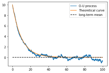
Let the mean-reversion strength by \(\mu = 0.1\) and the diffusion \(\sigma = 0.2\). Choose a total time over to integrated, in this case, over a total time of \(100\) units, with a time step of \(0.001\) (or \(1000\) Hertz). To generate Ornstein—Uhlenbeck stochastic trajectory with an Euler–Maruyama integration method, use

import numpy as np
import matplotlib.pyplot as plt

# integration time and time sampling
t_final = 100
delta_t = 0.001

# The parameters theta and sigma
mu = 0.1
sigma = 0.2

# The time array of the trajectory
time = np.arange(0, t_final, delta_t)

# Initialise the array y
X = np.zeros(time.size)

# We will start with an initial condition far from zero
X[0] = 10

# Generate a Wiener process
dw = np.random.normal(loc = 0, scale = np.sqrt(delta_t), size = time.size)

# Integrate the process
for i in range(1,time.size):
    X[i] = X[i-1] - mu*X[i-1]*delta_t + sigma*dw[i]

# plot the trajectory of y
plt.plot(time, X, label='O-U process')

# plot the 'theoretical' curve for an ODE
plt.plot(time, X[0]*np.exp(-mu*time), label='Theoretical curve')

# and the mean around zero
plt.plot(time, np.zeros(time.size), '--', color = 'black', label='long-term mean')

plt.legend()

Ambiguities and field-specific meaning

In different fields stochastic equations are represented differently. For example, a common conception of Markov processes in physics is known as the Langevin equation. Take \(x(t)\) representing the position of a particle. The Langevin equation is given by

\[ \frac{d x(t)}{d t} = -\frac{\partial V(x)}{\partial x} + \epsilon \xi(t), \]

where \(V(x)\) is an associated potential and \(\xi(t)=\frac{d W(t)}{d t}\) is a Gaussian white noise (or Wiener noise). Understandably from a mathematical point-of-view the operation of differentiating a Gaussian noise is not well defined, as this noise is almost surely nowhere differentiable.

It the mathematical literature it is more common to represent a stochastic differential equation in the differential form

\[ d X_t = a(X_t,t)d t + b(X_t,t) dW(t), \]

where a considerable care is put into what form of integration is needed to integrated \(dB(t)\). This is particularly more complicated with more sophisticated types of noise.

References

AitS08

Yacine Aït-Sahalia. Closed-form likelihood expansions for multivariate diffusions. The Annals of Statistics, 36(2):906–937, 2008.

Sin06

Hermann Singer. Moment equations and hermite expansion for nonlinear stochastic differential equations with application to stock price models. Computational Statistics, 21(3):385–397, 2006.

Authors

Houda Yaqine, Leonardo Rydin Gorjão