The Curse of Dimensionality in scRNA Data (draft)#
Part of a series: Uncertainty in scRNA experiments.
Follow reading here
Introduction#
Since the discovery of RNA sequencing [Nagalakshmi et al., 2008], lots of technological and algorithmic progresses have been made. With technological advances, we refer to the fact that better sequencers, improved protocols and more accurate quality measures produce more detailed and more reliable data for more biological cells. On the other hand, algorithmic progress means the methods required to handle these continuously evolving data adapt, too. Take, for instance, the Dirichlet process mixture model as described in this article. Here, Gibbs sampling uses exchangability of observations to loop over all cells in every MCMC iteration. Consequently, the evaluation time of such an iteration increases with the sample size. One should not hope that this issue will be solved with computational advances since both sides, the data generation and analysis, are equally affected by Moore’s law. This article introduces and compares two Markov chain Monte Carlo sampling variants in order to evaluate their applicability to high-dimensional data. Moreover, it includes results of a simulational study to visualize the impact of data dimensions and distributional forms.
Gibbs sampling for high-dimensional data#
Although parallelizations of the Gibbs sampling scheme have been researched, e.g. by [Chang and Fisher III, 2013], the potential computational gains are mathematically limited [Gonzalez et al., 2011] and susceptible to pitfalls [Gal and Ghahramani, 2014]. Furthermore, conditional sampling suffers from clusters which are ‘close’ in the sense that they have similar cluster-specific parameters [Jain and Neal, 2012]. Especially in scRNA data, it is likely that clusters differ only with respect to the expression levels of a few genes and hence parameters are indeed similar. The challenge for Gibbs updates with this kind of data is the fact that it needs to surpass a low probability region when splitting such ‘close’ clusters.
Split-Merge sampler#
To overcome the abovementioned shortcomings of Gibbs sampling, [Jain and Neal, 2012] developed a Metropolis-Hastings sampler which reassigns multiple data points at once in so-called split and merge moves. Conceptually, this sampler picks two cells at random and either merges their clusters (if the cells were in different clusters before) or splits it (if the cells were in the same cluster), respectively. The promising computational advantage is that ‘close’ clusters can theoretically be told apart in a single iteration. Analogously, unncessary subclusters of an actually homogenous subpopulation can be merged as such in a single iteration. As always, the improvements of the split-merge sampler are no free lunch. They come with the price of acceptance-rejection steps to ensure the detailed balance condition. Thus, it is crucial that proposed moves yield high probability regions to be accepted frequently. There is only one way to merge two clusters, but plenty of possible cell allocations for a split. Hence, finding a suited allocation provokes the bigger challenge and requires additional computations. The authors propose to run few restricted Gibbs iterations on the cells in the selected cluster. Doing so, results in higher acceptance rates but may impose a computational bottleneck because evaluation time of the marginal distribution within each Gibbs iteration often depends on the feature space. For instance, the marginal of the conjugate multinomial-Dirichlet model depends on the logarithms of gamma functions applied to every cell count which scales quite poorly. However, by now parallelized and distributed (across computing machines) variants of this sampling approach have been developed. Nevertheless, the question remains whether the split-merge sampler really solves the curse of dimensionality.
Simulational study#
This section sheds light on the effects that the following scenarios have on Gibbs and split-merge sampling.
inreasing feature space \(G\)
increasing amount of clusters \(K\)
model misspecification
Data sets have been simulated in R following this pseudo-algorithm
Algorithm 1 (scRNA data-simulation)
Inputs Given the cells per cluster (\(N\)), features per cell (\(G\)), clusters (\(K\)) and data generating process (\(f\))
Output Simulated data sets \(C \in \mathbb{N}_0^{NK,G}, \tilde C \in \mathbb{R}^{NK,G}\)
Sample \(\theta\sim Dir(1, repeat(1/G, G))\)
for each k in 1:K
Adapt \(\theta^{(k)}\) from \(\theta\)
for each i in 1:N
Sample \(p \sim Dir(a, \theta^{(k)})\)
Sample \(C_{k,i} \sim f(p)\)
\(\tilde C_{k,i} = log(\frac{C_{k,i}\cdot 10000}{\sum_g C_{k,i}}+1)\) #Normalize C
The number of cells per cluster has been fixed to \(N=100\) throughout this study\footnote{Please note that this does not represent a finite mixture model exactly. The choice has been made back then for computational ease (no cluster imbalances).}. The cluster-specific expression levels have been derived by random changes in \(\sqrt{G}\) entries of \(\theta\). The normalization is often carried out to account for batch effects and justify the assumption of normality of the data afterwards. Hence, this study considers two different data generating processes, the normal distribution (for normalized data \(\tilde C\)) and the multinomial distribution (for the count data \(C\)). Please note that normality is assumed for the normalized data and \(C\) must be derived by reversing the last line, respectively. The following graphic shows that this procedure is indeed valid in the sense that one can transform the multinomial counts (black) into normally distributed variables (blue) and vice versa. However, the variances of the normal distributions must be chosen carefully.
To compare the algorithms, the following three evaluation metrics have been applied to every clustering result.
adjusted Rand index
closeness to the true number of clusters \(K\)
evaluation time per iteration
The adjusted Rand index compares the amount of data points which share a common group (with the true cluster membership) to those which are different. The resulting index lies in the interval \([0,1]\) and a higher Rand index indicates better clustering. The class labels of the very last MCMC iteration have been used for this. It is noteworthy, that the Rand index becomes exactly zero when a clustering algorithm predicts for a homogenous population (one single cluster) more than one cluster. The higher the amount of true subpopulations, the less sensitive is this metric to an over-/underestimation of \(\hat K\). The second metric, closeness, accounts for this behavious and is defined as the relative frequency of MCMC iterations in which the assumed number of clusters is close to the actual value. More precisely is this the case, whenever \(\hat K \in \{K-1,K,K+1\}\). Lastly, two models may have vastly different computational costs (e.g.\ for the evaluation of the marginal distribuion) which may depend on \(N, G, K\).
Impact of the feature space#
By features we refer to the amount of columns in the observed count matrix \(C\). In a regression model, more features may provide more information and could lead to a better model (the curse of dimensionality with respect to model selection). Here, the computational time grows linear in \(G\) since the corresponding row vectors of \(C\) are fed into the marginal distribution. Moreover, the probability mass allocated among the genes, \(\theta \in [0,1]^G\), is constant. Thus several genes will have smaller expression probabilites (\(\exists g: \theta_g \to 0\)). If the data generating process is multinomial, such features will have low expressions with low variabilty and are overall less informative (i.e. \(\theta_g\to 0 \Rightarrow \mathbb{E}(C_g) \land \mathbb{V}(C_g)\to 0\)). Furthermore, the proportion of relevant features to differentiate clusters dicreases with increasing \(G\) because only \(\sqrt{G}\) random genes are altered per cluster.
The dashed lines in Fig. 66 indicate that evaluation times shoot up with larger feature spaces. Moreover, the Split-merge sampler appears to be more costly than the Gibbs counterpart. This was expected since every iteration of a Split-merge sampler includes a final Gibbs scan in addition to the split or merge move. The number of Markov chain iterations in which the samplers were close to the true number of clusters diminish quickly for larger feature spaces. This is true for all but the Split-Merge sampler with the correctly specified model (light yellow line). Hence, the impact of model missoecification and poor sampler choices apparently become more severe for high-dimensional data.
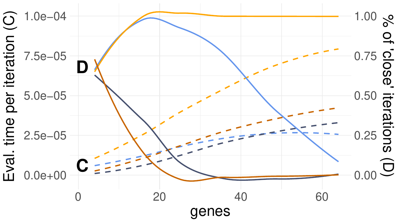
Fig. 66 Evaluation time (dashed lines) and closeness (solid) w.r.t. the number of detected clusters of Gibbs (blue) and Split-merge (yellow) sampling.#
Impact of the number of clusters#
More clusters lead to larger sample sizes in this simulation. Nonetheless, we cannot learn more about any particular cluster since the cluster size was chosen to be constant with \(N=100\). The boxplots in the left panel of Fig. 67 indicate the impact of increasing clustering complexity on a correctly specified model. Since the Rand indices of the Split-merge sampler slowly decreases, additional clusters seem to pose a more challenging scenario. The low Rand indices of the Gibbs sampler (blue boxes) emphasize that either the chains have not converged yet or the approach is not capable to cluster this data whatsoever. Interestingly, the boxes indicate not further suffering of Gibbs from additional clusters. Apparently, the choice of the sampler and model misspecification (right panel of the Fig. 67) have a larger impact on the clustering accuracy than the number of clusters.
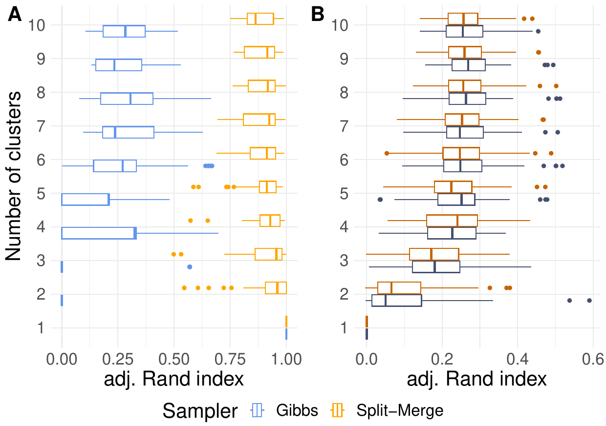
Fig. 67 Comparison of Gibbs and Split-merge sampling approaches using the Multinomial-Dirichlet (A) or independent conjugate normal (B) model, respectively on various feature spaces.#
Impact of model misspecification#
What happens if our modelling assumptions do not reflect the data is an ongoing research question. Even minor differences, such as assuming a normal distribution instead of a heavier-tailed t-distribution, may lead to undesirable behaviour (e.g. increased sensitivity to outliers). This issue affects scRNA analyses as well. The following questions will be covered in this section:
Should counts be modelled jointly multinomial or gene-specific negative binomial?
Should normalized counts be modelled with normal distributions?
Several distributional choices exist to model count data. The reasoning behind the multinomial model is often its entropy. In plain words, this distribution is the most flexible way to allocate \(n\) objects into \(G\) buckets. Here, two important assumptions are implicitly made. Firstly, the expected proportion of objects for every bucket shall be constant and denoted by (the only) parameter \(\theta\). Secondly, the variance of objects in every bucket is determined by this parameter, too. Hence, we cannot model a gene with low counts \(\theta_g \to 0\), but a large variance/rare high counts, even though exactly this overdispersion has been observed empirically. The negative binomial distribution overcomes this problem, but the added modelling flexibility could also lead to merged overlapping clusters. It worth pointing out, that the negative binomial distribution can only handle overdispersion, but is incapable to model variances smaller than in the multinomial model.
Normal distributions have a seperate parameter for the variance, too, and are thus equally suited for overdispersion. Moreover, count normalization is often applied in practice anyway to account for batch effects (vastly different sum of counts across cells) and huge values. Still open is the question how well a normal distribution fits to the transformed counts if these were originally simulated with one of the count distributions mentioned above. Vice versa, one could ask how well a multinomial model captures counts which are derived by back-transforming something normally distributed? The following graphic highlights that this question is not trivial, but depends on the particular characteristics of the data generating process. The graphic is based on \(1000\) cells which have only \(G=3\) genes. The first one has a low expression value and the remaining two are quite similar, i.e. \(\theta = (0.01, 0.46, 0.53)\).
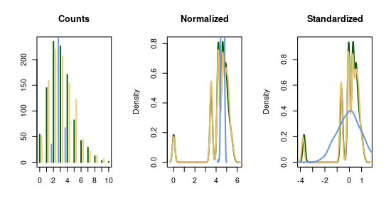
Fig. 68 Evaluation time and closeness w.r.t. the number of detected clusters of Gibbs and Split-merge sampling.#
If the expected counts, \(n\cdot \theta_g\), are large enough, then the normal approximation works well in the sense that the normal distribution (blue) and normalized counts (green) in the center panel look similar. The same holds in the left panel for the counts. If, however, the expression is low and especially when only few different count values are observed (e.g. \(C_{i,g} \leq 4, \forall i\)), then the normalization will yield a multimodal distribution in which each mode represents a transformed integer. This behaviour will persist whenever small counts are observed because the normalization is non-linear with the largest “jumps” for small counts (i.e. \(f(c) - f(c-1) > f(c+1)-f(c), \forall c\)). Obviously, dropouts only add up to this problem.
References#
- CFI13
Jason Chang and John W Fisher III. Parallel sampling of dp mixture models using sub-cluster splits. Advances in Neural Information Processing Systems, 2013.
- GG14
Yarin Gal and Zoubin Ghahramani. Pitfalls in the use of parallel inference for the dirichlet process. In 31st International Conference on Machine Learning, ICML 2014, volume 2, 1437–1445. 2014.
- GLGG11
missing journal in Gonzalez2011ParallelTrees
- JN12(1,2)
Sonia Jain and Radford M. Neal. A Split-Merge Markov chain Monte Carlo Procedure for the Dirichlet Process Mixture Model. https://doi.org/10.1198/1061860043001, 13(1):158–182, 3 2012. URL: https://www.tandfonline.com/doi/abs/10.1198/1061860043001, doi:10.1198/1061860043001.
- NWW+08
Ugrappa Nagalakshmi, Zhong Wang, Karl Waern, Chong Shou, Debasish Raha, Mark Gerstein, and Michael Snyder. The transcriptional landscape of the yeast genome defined by RNA sequencing. Science, 320(5881):1344–1349, 2008.