Quasi-Monte Carlo Method

Part of a series: Monte Carlo Method.

Follow reading here

Uncertainty quantification deals with models which has uncertain random inputs or parameters. In case of forward uncertainty propagation, Monte Carlo method is the only option due to high dimensinality of a problem. Monte Carlo method computes the mean and variance of the output of the model given the uncertain inputs and/or parameters. For simplicity, assume a model as numerical with uncertainty in its input varaiables. However, the efficiency of the Monte-Carlo method can be improved using other sampling techniques. This articles gives an overview of Monte Carlo (MC) and Quasi-Monte Carlo (qMC) method. If \(u(Z)\) is the model response i.e (data-to-solution map) and the interested quantity of interests (QoIs) related to \(u(Z)\), are \(E[u(Z)], Var[u(Z)]\) then in mathematical terms the the expected value is written as the integral,

\[ E[u(Z)] = \int_{[0,1]^d} \underbrace{u(z) \rho(z) }_{g(z)} dz. \]

In the MC method, one simply take \(N\) random samples \( Z^{i}\) of the input and the empirical mean is computed as follows,

\[ E(u) \approx \bar u_h^{(N)} := \frac{1}{N} \sum_{i=0}^{N} u_h (Z)^{i}, \]

where \(h\) can be a discretization parameter. This formulation brings up a question of how to select the number of samples \(N\) for a given \(h\) at a desired accuracy. This is answered by using the mean squared error (MSE)

\[ \text{MSE} := E \left( \left| E[u] - E_N[u_h]\right)^2 \right) = \underbrace{\left( E[u] - E_h[u_h] \right)^2}_{\text{squared bias}} + \underbrace{\frac{V[u_h]}{N}}_{\text{statistical error}}. \]

In above equation, the MSE is governed by two factors, i.e. bias and variance which a statistical quantity. The bias term is governed by the discretization parameter of the underlining numerical method \(h\) whereas the variance is due of the number of samples \(N\). The variance is estimated as,

\[ V[u] \approx \frac{1}{N-1} \sum_{i=0}^{N} (u^{(i)} - \bar u ^{N})^2. \]

The root mean square error of MC (unbiased) is given as,

\[ ( E [ (\epsilon_N (u))^2 ] )^{\frac{1}{2}} = \sqrt{\frac{V[u]}{N}}. \]

The convergence rate of MC then is \( \frac{1}{ \sqrt{N}}\). This can be improved to \((logN)^d \frac{1}{N} \) by using quasi-random numbers. In the literature there are many sampling techniques that can be used to sample the quasi-random numbers. Here, four major sampling techniques are briffly discussed. For detailed reading see [Smith, 2014]. Monte-Carlo method uses pesudo-random numbers that converges with convergence rate \(O(1/N^{1/2})\) see [Caflisch and others, 1998]. However this convergence rate can be improved by using other, above defined methods.

• Quasi-random Monte-Carlo sampling

• Latin hyper-cube sampling

Quasi Monte-Carlo Method (QMC)

The main idea behind the quasi Monte-Carlo method is to use low discrepancy sequences LDS [Niederreiter, 1978] for the random varaible. The LDS is briefly defined below. In practice Sobol’ sequences [Burhenne et al., 2011] are used. Similar to the Monte-Carlo method, QMC method is given by,

\[ E(u) \approx \bar u_h^{(N)} := \frac{1}{N} \sum_{i=0}^{N} u_h (\xi)^{i}, \]

where \({Z^i}\), in this case are chosen as LDS sample points. The Koksma-Hlawka theorem [Brandolini et al., 2013] gives an upper bound on the integration. The Koksma-Hlawka inequality is given as,

\[ \varepsilon \leq V(u)D_N^{*}, \]

where \(V(f)\) is the variation in \(f(\xi)\) and \(D_N*\) is the discrepency in the sampled points. The variation in \(f(\xi)\) is given by (for simplicity in 1D),

\[ V(u) = \int_{H} |\frac{du}{d\xi}|d\xi. \]

In practice, the QMC gives the convergence rate of \(O(N^{-\alpha})\) for \(0 < \alpha \leq 1\). So by using the QMC with LDS the standard Monte Carlo method can be made more efficient. [Caflisch and others, 1998]

Low Discrepency Sequences (LDS)

Discrepency is a quantitative measure of the highest and lowest density of points. Roughly speaking, low discrepency means that the points or random samples are spread through the sample space or there are less empty spaces as compared the number of points. Quantitatively, it explains the deviation of sampled points from a uniform distribution. In precise mathematical form, the LDS is given by,

\[ D_N(P) = \frac{N_{Q(P)}}{N} - m(Q(P)), \]

where \(N\) is the total number of sampled points in the hyper cube \(H^n\), \(Q(P)\) is a subset of \(H^n\) with \(N_{Q(P)}\) number of points inside it. \(m(Q(P))\) is the volume of \(Q(P)\). In practice, the LDS will give better convergence rate [Helton and Davis, 2003].

Latin Hyper Cube Sampling (LHS)

Similar to the QMC, LHS also gives better efficiency by using the advantage of stratified sampling. The main idea is to use stratified sampling to reduce the variance in the Monte-Carlo error estimate. The algorithm which is used to generate this type of random variables is given by,

\[ \xi_i^k = \frac{\pi_k(i)-1 + U_i^k}{N}, i= 1,...N; k=1,...n. \]

Here \(U_i^k\) are independent-identically-distribution (i.i.d) random numbers between \([0,1]\). To understand this algorithm generate \(n\) sequences \({\xi_i^1}\), \(i=1,...,N\), in \(H^1\) (since hyper cube has \(n\) dimensions). These sequences are then paired together to form \(N\) samples of \(n\)-dimensional random numbers. See the figure below. For further detail see [Helton and Davis, 2003]. The different example of sampling methods in 2D are presented below in Fig. 20 and Fig. 21.

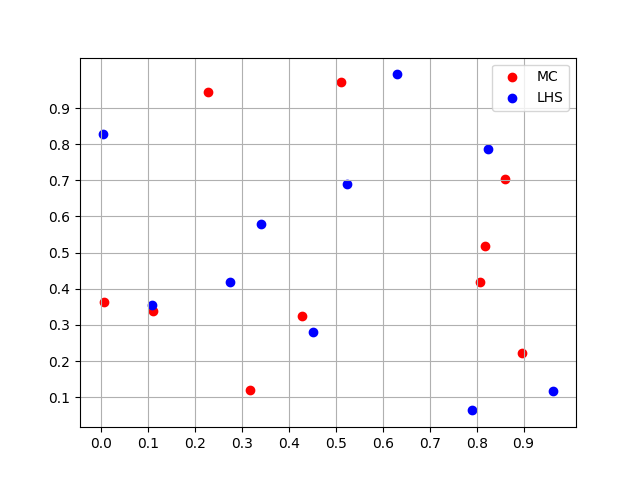
Fig. 20 2D example of Latin Hypercube Sampling

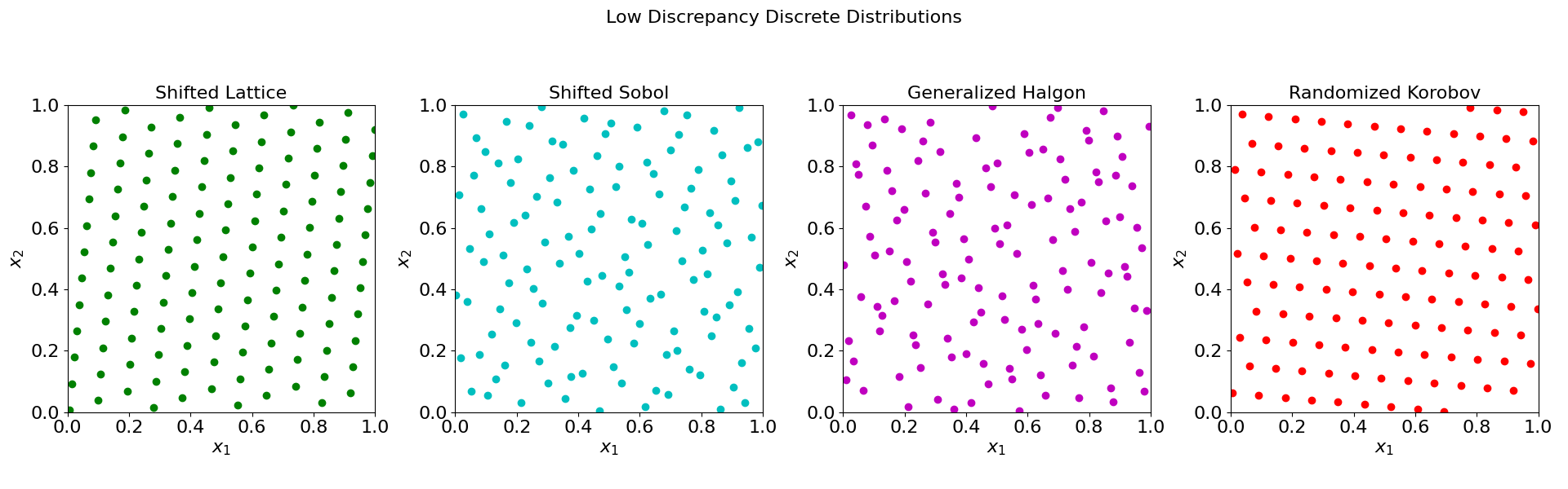
Fig. 21 2D examples of Low Discrepancy Discrete Distributions

Software

1. QMCPy: Quasi-Monte Carlo in Python

   • Description: QMCPy is a Python library designed for Quasi-Monte Carlo methods. It provides a range of functionalities for generating low-discrepancy sequences, conducting QMC integration, and analyzing results.

   • Link: QMCPy Documentation

2. lhsmdu: Latin Hypercube Sampling in Python

   • Description: The lhsmdu package is a Python implementation specifically focused on Latin Hypercube Sampling. It allows users to generate Latin hypercube samples efficiently.

   • Link: lhsmdu on PyPI

References

BCGT13

Luca Brandolini, Leonardo Colzani, Giacomo Gigante, and Giancarlo Travaglini. On the koksma–hlawka inequality. Journal of Complexity, 29(2):158–172, 2013.

BJH11

Sebastian Burhenne, Dirk Jacob, and Gregor P Henze. Sampling based on sobol’sequences for monte carlo techniques applied to building simulations. In Proc. Int. Conf. Build. Simulat, 1816–1823. 2011.

C+98(1,2)

Russel E Caflisch and others. Monte carlo and quasi-monte carlo methods. Acta numerica, 1998:1–49, 1998.

HD03(1,2)

Jon C Helton and Freddie Joe Davis. Latin hypercube sampling and the propagation of uncertainty in analyses of complex systems. Reliability Engineering & System Safety, 81(1):23–69, 2003.

Nie78

Harald Niederreiter. Quasi-monte carlo methods and pseudo-random numbers. Bulletin of the American mathematical society, 84(6):957–1041, 1978.

Smi14

Ralph C Smith. Uncertainty quantification: theory, implementation, and applications, volume 12 of computational science & engineering. Society for Industrial and Applied Mathematics (SIAM), Philadelphia, PA, 2014.

Author

• Maqsood Mubarak Rajput