Monte-Carlo Method

Monte-Carlo Method#

This article is part of a series: Monte Carlo Methods. The following aspects are covered

Methods and Applications:
Use Cases

Introduction#

The Monte-Carlo method is a non-intrusive method to propagate uncertainties through a given code. Monte-Carlo treats the given code as a black box which is evaluated at random samples of the input probability distribution. Outputs at these realizations are then used to approximate quantities such as expectation or variance. The workflow reads

Generate a sample of the input random variable $Z\in\mathbb{R}^d$, distributed according to $f$.
Second, run the model with these parameters $Z^{(i)}$ where $i=1,\cdots,N$. This generates samples of the output, which we denote by $u\left( Z^{(i)}\right)$.
Third, compute the QoIs from this sample, e.g, $\mathbb{E}[u(Z)]\approx\frac{1}{N}\sum_{i=1}^{N}u\left( Z^{(i)}\right)$

Description#

In uncertainty quantification (UQ), mathematical models are provided with random input $ Z \in \mathbb{R}^{d}$. If $u(Z)$ is the model response i.e (data-to-solution map) and the interested quantity of interests (QoIs) related to $u(Z)$, are $E[u(Z)], Var[u(Z)]$ then in mathematical terms the the expected value is written as the integral,

\[ E[u(Z)] = \int_{[0,1]^d} \underbrace{u(z) \rho(z) }_{g(z)} dz. \]

In the MC method, one simply take $N$ random samples $ Z^{i}$ of the input and the empirical mean is computed as follows,

\[ E(u) \approx \bar u_h^{(N)} := \frac{1}{N} \sum_{i=0}^{N} u_h (Z)^{i}, \]

where $h$ can be a discretization parameter. This formulation brings up a question of how to select the number of samples $N$ for a given $h$ at a desired accuracy. This is answered by using the mean squared error (MSE)

\[ \text{MSE} := E \left( \left| E[u] - E_N[u_h]\right)^2 \right) = \underbrace{\left( E[u] - E_h[u_h] \right)^2}_{\text{squared bias}} + \underbrace{\frac{V[u_h]}{N}}_{\text{statistical error}}. \]

The MSE is governed by two factors, i.e. bias and variance which a statistical quantity. The bias term is governed by the discretization parameter of the underlining numerical method $h$ whereas the variance is due of the number of samples $N$. The variance is estimated as,

\[ V[u] \approx \frac{1}{N-1} \sum_{i=0}^{N} (u^{(i)} - \bar u ^{N})^2. \]

The root mean square error of MC (unbiased) is given as,

\[ ( E [ (\epsilon_N (u))^2 ] )^{\frac{1}{2}} = \sqrt{\frac{V[u]}{N}}. \]

The convergence rate of MC then is $\frac{1}{ \sqrt{N}}$. This can be improved to $(logN)^d \frac{1}{N} $ by using quasi-random numbers. In the literature, variance reduction techniques are also used in order to reduce the cost of computation. Multilevel Monte Carlo (MLMC) method is one of those methods.

Lemma: MSE complexity analysis MC (error vs cost)#

Suppose that:

$\left| E \left[ u - u_h \right] \right| = \mathcal{O}\left(h^{\alpha}\right)$
$V[u_h] = \mathcal{O}(1)$
$\text{cost} \left( u_h^{(i)}\right) = \mathcal{O}(h^{-\gamma})$

Achieving $MSE \leq \epsilon^2$ requires $N = \mathcal{\epsilon^{-2}}$ and $h = \mathcal{\epsilon^{1/\alpha}}$, resulting in the computational cost $= N cost(u_h) = \mathcal{O}\left( \epsilon^{-(2+ \gamma / \alpha)} \right)$.

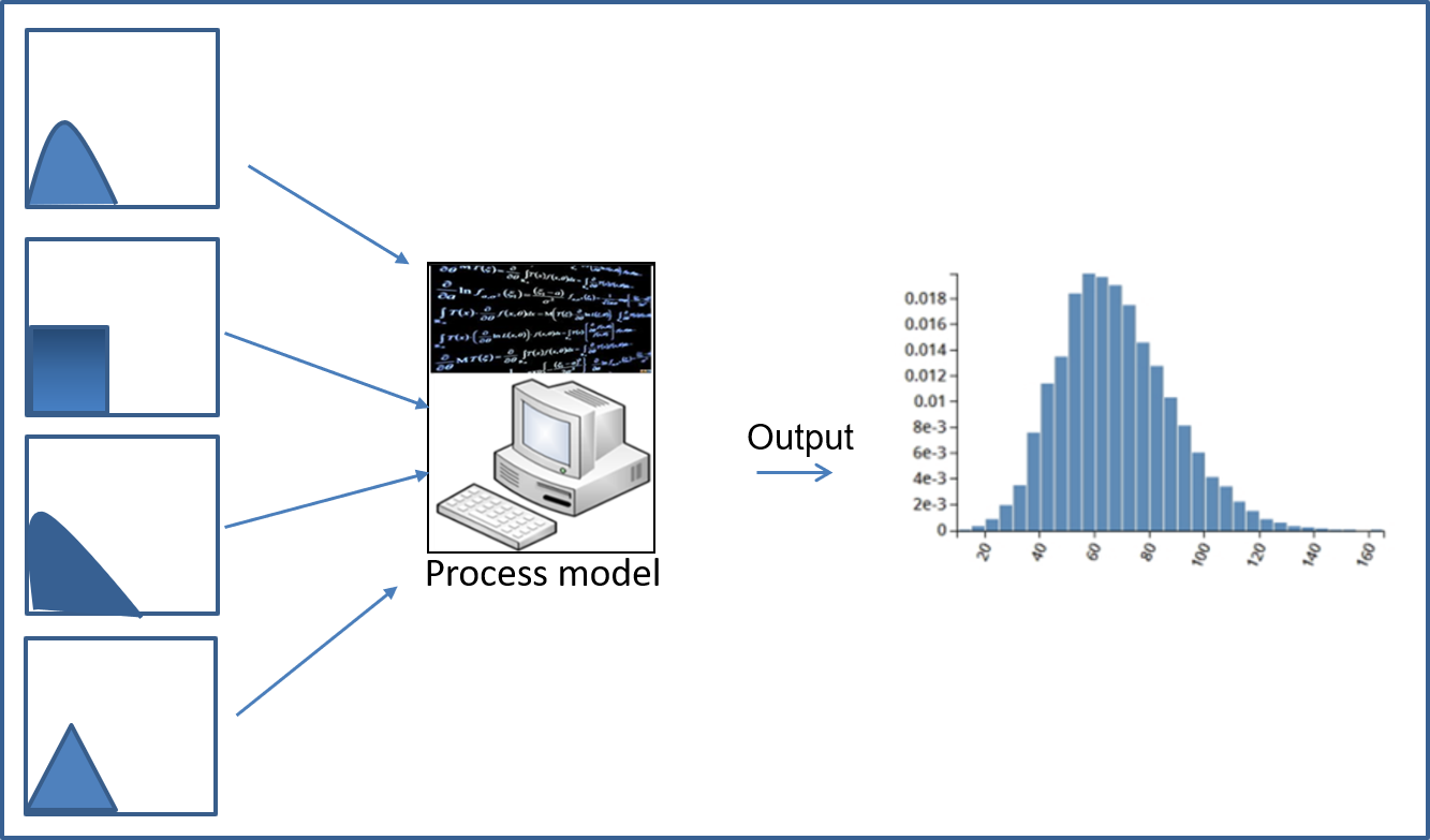
Fig. 17 Example illustration of Monte-Carlo#

Examples#

Use of Monte-Carlo for $\pi$ approximation: The value of $\pi$ can be estimated by uniformly sampling points in the interval $[0,2]\times[0,2]$ and counting the ratio of the number of points falling into the circle (red) to the total number (red + blue points).

Fig. 18 Use of Monte-Carlo for $\pi$ approximation#

Approximation of $\mathbb{E}[f]$ with Monte-Carlo: Let $\xi$ be a random variable with probability density $f_{\Xi}:\Theta\rightarrow\mathbb{R}_+$ and $f$ be a function $f:\Theta\rightarrow\mathbb{R}$. We wish to determine the expectation of $f$, which reads $\mathbb{E}[f]=\int_{\Theta}f(\xi)f_{\Xi}\,d\xi$. The expectation is approximated by generating samples according to the distribution $f_{\Xi}$ and evaluating $\mathbb{E}[f]\approx\frac{1}{N}\sum_{i=1}^{N}f\left( \xi^{(i)}\right)$. The values of $f(\xi^{(i)})$ are determined by treating the implementation of $f$ as a black box, which is evaluated at all $N$ sample points.

Fig. 19 Approximation of $\mathbb{E}[f]$ with Monte-Carlo#

Remarks#

Parts of the material presented in this entry have been taken from the Uncertainty Quantification lecture notes of Martin Frank.

Authors#

Maqsood Mubarak Rajput, Jonas Kusch