Representation of a Reaction System by Ordinary Differential Equations

Part of a series: Uncertainty Quantification for a Dynamical Model.

Follow reading here

The preceding article shows how the dynamics of a reaction system can be modeled. The chemical master equation (CME) describes the temporal evolution of the state distributions of a Markov jump process (MJP). Sample paths of an MJP are generated by Gillespie’s algorithm. However, the CME admits, in general, no analytic solution. Besides, Gillespie’s algorithm can be computational costly, if a large number of individuals or fast successive reactions induce a large number of reactions [Hasenauer, 2013]. Therefore, approximations are commonly used to circumvent this issues. This article focuses on a representation in terms of a system of ordinary differential equations (ODEs). A system of ODEs constitutes a deterministic model. It assumes that the number of individuals of all objects are sufficiently large such that random fluctuations of system entities are negligible. More details on ODE approximations of reaction systems can be found, for example, in [Hasenauer, 2013, Gratie et al., 2013, Lei, 2021]. Moreover, there are numerous mathematical textbooks that introduce ODEs formally, see e.g. [Adkins and Davidson, 2012, Hale, 2009].

Within this article, if not stated otherwise, we again adopt the notation from the preceding articles about reaction systems and their stochastic representation.

We assume that the number of individuals of objects \(X_i\), for \(i=1,\dots,N\), is “large”. It allows us to consider the concentrations of objects

\[ \begin{align*} x_i(t)=\frac{X_i(t)}{V}\in\mathbb{R}_+,\quad\text{for }i=1,\dots,N,~t\ge0, \end{align*} \]

that can in turn be regarded as continuous-valued quantities for a total system volume \(V\in\mathbb{N}\). We denote by \(x(t)=(x_1(t),\dots,x_N(t))\) the vector of all concentrations at time \(t\). In addition to that, the assumption above further enables to use an approximation for the (adapted) propensity function of an reaction \(R_r\), for \(r=1,\dots,M\), by

\[ \begin{align*} \tilde{a}_r(x(t))\approx \tilde{c}_r\prod_{i=1}^Nx_i(t)^{s_{ir}}, \end{align*} \]

where \(\tilde{c}_r\) and \(s_{ir}\) are the corresponding (adapted) reaction rate constants and stoichiometric coefficients, respectively. Note that we need to use converted versions \(\tilde{a}_r\) and \(\tilde{c}_r\) of \(a_r\) and \(c_r\), respectively, due to the scaled concentrations \(x_i(t)\) that we consider from now on. Appropriate conversions are, for example, given in [Hasenauer, 2013, Lei, 2021].

The state dynamics can then be described by the system of ODEs

(4)\[ \begin{align} \frac{\mathrm{d} x(t)}{\mathrm{d} t}=S\tilde{a}(x(t)),\quad x(0)\in\mathbb{R}_+^N, \end{align} \]

where \(S\in\mathbb{Z}^{N\times M}\) again denotes the stoichiometric matrix and \(\tilde{a}(z)=(\tilde{a}_1(z),\dots,\tilde{a}_M(z))\). Equation (4) is also known as reaction rate equation (RRE). In [Gillespie, 2000, Lei, 2021], the authors show more formally that the RRE indeed represents the CME. Other approximation methods of the CME, e.g. an approximation by stochastic differential equations, system size expansion or moment closure methods, are discussed in [Loskot et al., 2019].

We conclude this article with an ODE representation of the running example from the preceding articles.

Example

In this example, the propensity functions for the concentrations do not alter. It holds that

\[ \begin{align*} \tilde{a}_1(x(t))=c_1,\qquad \tilde{a}_2(x(t))=c_2x_1(t),\qquad \tilde{a}_3(x(t))=c_3x_2(t). \end{align*} \]

The RRE is then given by

\[\begin{split} \begin{align*} \mathrm{d} x_1(t)&=\left(c_1-c_2x_1(t)\right)\mathrm{d} t, \quad x_1(t_0)=x_1(0),\\ \mathrm{d} x_2(t)&=\left(c_2x_1(t)-c_3x_2(t)\right)\mathrm{d} t, \quad x_2(t_0)=x_2(0). \end{align*} \end{split}\]

Fig. 23 displays in colours the deterministic solution of the 2-dimensional RRE approximated with the Euler method, the deterministic version of the Euler-Maruyama method for stochastic differential equations.

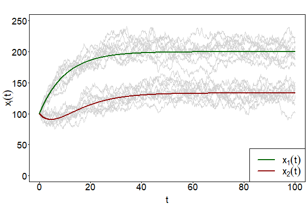
Fig. 23 An approximate solution of the 2-dimensional RRE with \(c_1=20,~c_2=0.1,~c_3=0.15,~x_1(0)=100\) and \(x_2(0)=100\). The green and red curve correspond to the state variables \(x_1(t)\) and \(x_2(t)\), respectively. Random trajectories of the underlying MJP are depicted in grey.

References

AD12

William A. Adkins and Mark G. Davidson. Ordinary Differential Equations. Springer, 2012.

Gil00

Daniel T. Gillespie. The chemical Langevin equation. Journal of Chemical Physics, 113:297–306, 2000.

GIP13

Diana-Elena Gratie, Bogdan Iancu, and Ion Petre. ODE analysis of biological systems. Formal Methods for Dynamical Systems, pages 29–62, 2013.

Hal09

Jack K. Hale. Ordinary Differential Equations. Dover Publications, 2009.

Has13(1,2,3)

Jan Hasenauer. Modeling and parameter estimation for heterogeneous cell populations. University of Stuttgart (PhD Thesis), 2013.

Lei21(1,2,3)

Jinzhi Lei. Systems Biology: Modelling, Analysis, and Simulation. Springer, 1 edition, 2021.

LAM19

Pavel Loskot, Komlan Atitey, and Lyudmila Mihaylova. Comprehensive review of models and methods for inferences in bio-chemical reaction networks. Frontiers in Genetics, 2019.

Authors

Julian Wäsche