Polynomial Chaos Expansion#
Polynomial chaos expansion (PCE) is a statistical method for approximating the output of a complex system as a sum of orthogonal polynomials with random coefficients. It is commonly used in uncertainty quantification and sensitivity analysis to propagate uncertainty from the input parameters to the output quantities of interest [Cheng et al., 2020, Sudret et al., 2017, Wang et al., 2021]. More specifically, PCE is a spectral algorithm that can be seen as Fourier analysis for random variables of finite variance. This method approximates the probability density of the model output and determines uncertainty propagation in model-based computations. In general, PCE can reduce the number of samples used in the experiment design significantly, while providing a precise approximation of the model response. PCE provides a compact representation and highly accurate approximations of the output distribution, especially if the polynomial degree is sufficiently high. The output distribution is presented as the sum of orthogonal polynomials. This can be more computationally efficient than other methods, such as Monte Carlo simulation. Additionally, it is possible to directly compute the output distribution moments from the PCE coefficients. Furthermore, PCE can handle a wide range of input distributions, including continuous and discrete. It can be adapted to non-linear systems by using higher-degree polynomials [Cheng et al., 2020, Ghanem et al., 2017]. Within the UQ approach, PCE provides a probabilistic representation of the output distribution, which is useful for uncertainty quantification and sensitivity analysis. Moreover, the fast convergence rate of PCE is one of the main advantages over the classical approaches to determining the propagation of uncertainties [Ghanem et al., 2017]. For high-dimensional problems or when a large number of polynomials is required to achieve sufficient accuracy, however, the computational complexity becomes very high and eventually infeasible and the algorithm needs to be adjusted or changed. The choice of polynomial basis and the number of terms to include in the expansion for a particular system can be challenging, however, it has a significant impact on the results and the most appropriate model representing the system [Cheng et al., 2020, Ghanem et al., 2017]. PCE algorithms assume Gaussian input parameters, which limits their application to some types of data. Another limitation of PCE is polynomial approximation. This may not accurately capture the system’s behavior if it is highly non-linear or if the input distribution is not well represented by the polynomial basis [Cheng et al., 2020, Sobester et al., 2008].
Mathematical Presentation Of PCE#
The PCE of a random variable \(X\) is a decomposition of it into (potentially infinitely many) deterministic terms. These terms consist of deterministic coefficients \(a_k\) and the \(\phi_k\), such that
For practical application the infinite-dimensional representation is truncated to a smaller number of \(p\) coefficients, where \(p\) is set as small as possible while maintaining a sufficiently good approximation
The coefficients \(a_k\) of the PCE must be estimated in order to express the random quantities \(\mathcal{M}(\mathbf{X})\) via the orthogonal polynomials, which is one of the main challenges in PCE. The estimation of these coefficients \(a_k\) leads to two main types of PCE; intrusive and non-intrusive [Böttcher et al., 2021, Ghanem et al., 2017, Sobester et al., 2008]. The Intrusive PCE, where the algorithm directly alters the model equations or code under study by introducing the decomposition of the input quantity \(X\) directly to the model \(\mathcal{M}\) to create the PCE-overloaded model \(\mathcal{M}^{PCE} (X)\). The input PCE coefficients are then estimated via the projection approach, mainly the the stochastic Galerkin projection. Furthermore, using the PCE-overloaded model it is possible to directly retrieve the the coefficients of the random output quantity \(Y = \mathcal{M}(X)\) as can be seen in Figure Fig. 37a. For non-intrusive PCE approach, only deterministic evaluations of the original model are necessary, where the PCE coefficients are calculated in order to fit the original model. In this approach, the original model \(\mathcal{M}\) is considered as a black-box model. \(X\) samples are used to obtain \(X^{(i)}\) realizations via the evaluation of the model. This yields the observations \(y^{(i)}\), which will be used with the realizations to create the surrogate model \(\mathcal{M}^{PCE}\), as can be seen in Figure Fig. 37b.
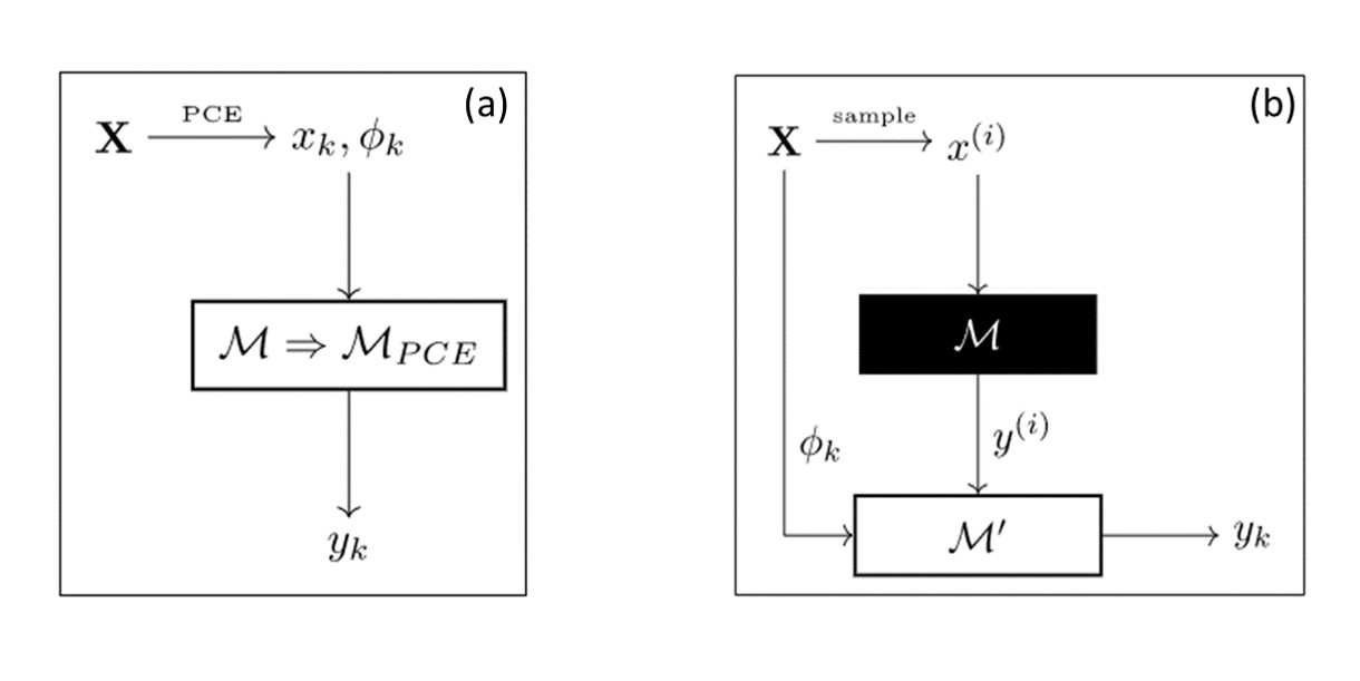
Fig. 37 Schematic of PCE (a) intrusive (b) non- intrusive (Image by:Adrian Grupp).#
Example#
In this code, we generate random values for three input parameters \((x_1, x_2, x_3)\) and evaluate the target function (\(target_function\)) using these input values to obtain the corresponding output (\(y\)).
{
import numpy as np
from sklearn.linear_model import LinearRegression
from sklearn.preprocessing import PolynomialFeatures

# Define the input parameters
x1 = np.random.uniform(0, 1, 100)  # Input parameter 1
x2 = np.random.uniform(0, 1, 100)  # Input parameter 2
x3 = np.random.uniform(0, 1, 100)  # Input parameter 3

# Define the target function to be approximated (example: f(x1, x2, x3) = x1 + 2*x2 + 3*x3)
def target_function(x1, x2, x3):
    return x1 + 2*x2 + 3*x3

# Evaluate the target function
y = target_function(x1, x2, x3)

# Create the input feature matrix
X = np.column_stack((x1, x2, x3))

# Define the degree of the polynomial expansion
degree = 2

# Perform polynomial feature expansion
poly = PolynomialFeatures(degree=degree) # PolynomialFeatures class from scikit-learn
X_poly = poly.fit_transform(X)

# Create and fit the linear regression model
model = LinearRegression()              # linear regression model
model.fit(X_poly, y)

# Predict using the surrogate model
x1_new = 0.5  # New input parameter 1
x2_new = 0.3  # New input parameter 2
x3_new = 0.2  # New input parameter 3

X_new = np.array([[x1_new, x2_new, x3_new]])
X_new_poly = poly.transform(X_new)

y_pred = model.predict(X_new_poly)

# Print the predicted output
print("Predicted output:", y_pred)

}
The output of this model is the predicted response of the fitted input parameters calculated using PCE model.
PCE Toolboxes Aand Libraries#
Several toolboxes and libraries are developed for PCE. These toolboxes and libraries are developed in MATLAB, Python, C++ etc. Here is some example of them :
MATLAB
Sergey Oladyshkin (2023). aPC Matlab Toolbox: Data-driven Arbitrary Polynomial Chaos (https://www.mathworks.com/matlabcentral/fileexchange/72014-apc-matlab-toolbox-data-driven-arbitrary-polynomial-chaos).
K. Sepahvand (2023). Coefficients of Polynomial Chaos Expansion (PCE) (https://www.mathworks.com/matlabcentral/fileexchange/73416-coefficients-of-polynomial-chaos-expansion-pce)
Luca Fenzi (2023). Robust stability optimisation of DDAE of retarded type (https://www.mathworks.com/matlabcentral/fileexchange/59627-robust-stability-optimisation-of-ddae-of-retarded-type)
UQLab (https://www.uqlab.com/kriging-user-manual)
Python
https://pypi.org/project/chaospy/4.2.3/
https://chaospy.readthedocs.io/en/master/
https://github.com/pygpc-polynomial-chaos/pygpc
https://chi-feng.github.io/pce-demo/
UQ[py]Lab (https://uqpylab.uq-cloud.io/)
Case Study#
See Modelling the Degradation of Biodegradable Implants for the application of PCE to model the complex degradation of biodegradable magnesium-based implants.
References#
- BottcherLF+21
Maria Böttcher, Ferenc Leichsenring, Alexander Fuchs, Wolfgang Graf, and Michael Kaliske. Efficient utilization of surrogate models for uncertainty quantification. PAMM, 20(1):e202000210, 2021.
- CLLZ20(1,2,3,4)
Kai Cheng, Zhenzhou Lu, Chunyan Ling, and Suting Zhou. Surrogate-assisted global sensitivity analysis: an overview. Structural and Multidisciplinary Optimization, 61:1187–1213, 2020.
- GHO+17(1,2,3,4)
Roger Ghanem, David Higdon, Houman Owhadi, and others. Handbook of uncertainty quantification. Volume 6. Springer, 2017.
- SFK08(1,2)
András Sobester, Alexander Forrester, and Andy Keane. Engineering design via surrogate modelling: a practical guide. John Wiley & Sons, 2008.
- SMW17
Bruno Sudret, Stefano Marelli, and Joe Wiart. Surrogate models for uncertainty quantification: an overview. In 2017 11th European conference on antennas and propagation (EUCAP), 793–797. IEEE, 2017.
- WWYC21
Kaiwen Wang, Yinan Wang, Xiaowei Yue, and Wenjun Cai. Multiphysics modeling and uncertainty quantification of tribocorrosion in aluminum alloys. Corrosion Science, 178:109095, 2021.
Contributors#
Maqsood Mubarak Rajput, Berit Zeller-Plumhoff