UQ in Surface Wave Tomography (Draft)#
Introduction#
The estimation of seismic hazard, exploitation of the underground for mineral resources, geothermal energy generation and storage, and understanding of geodynamic processes require knowledge and interpretation of the structure of the subsurface. Seismic tomography is a technique that uses model inference of seismic waves either directly or in combinations with secondary measurements (e.g., surface wave dispersion curves, travel times, and preprocessed traces) to characterize the Earth’s interior. The physical relation among measurements and Earth’s interior within these models are sometimes described by simplified schemes known as parameterisations so that one can construct a physical relation that predicts corresponding data. Fig. 81 shows an example that a simple layered model with a particular parameter set (e.g. velocity, density, and thickness of a layer) can reproduce simulated surface wave dispersion. The values of the parameters within these schemes are constrained by inversion of observation, thus, seismic tomography is a parameter estimation problem. Inversion is a way to invert the physical property parameters (e.g., velocity and density of subsurface rock) of the geological targets based on the geophysical model function.
Seismic inversion seeks optimal parameter values (e.g., velocity and density of subsurface rock) that match the seismic measurements or observations. In the pursuit of the optimal model with optimal parameter values, the majority of inversion procedures cycle through forward modeling and inversion, with the goal of minimizing the difference between the synthetic data and the observations. However, due to the insufficient data coverage, data noise, and nonlinearity of the physical relation, geophysical inverse problems are inherently non-unique, a large set of parameter values can fit the observed data well within their data uncertainties. The conventional optimization method which only gives one set of parameter values in the end has relied on regularization (i.e. additional terms of the objetive functions that punish large model perturbation). Regularization is used to tune the resolution and variance properties of the model. In geophysical models, higher resolution means the model can represent subtle variations in the properties being studied. For example, in seismic inversion, higher resolution might allow you to identify small-scale geological structures or anomalies within a larger region. Variance here refers to the degree of fluctuation or noise present in the model. High variance means that the model is highly sensitive to the noise in the data, which can lead to overfitting. By applying regularization, the complexity of the model can be control manually and prevent it from overfitting while still maintaining sufficient resolution to capture important features. To create a stable solution, the estimated uncertainty of individual model parameters is often underestimated due to the strong trade-off between model resolution and variance. As geophysical and geological inference inherently rely heavily on interpreted models, it is crucial to adequately communicate their uncertainties to avoid misinterpretations.
Surface waves are a type of seismic energy that travels along the Earth’s surface. The benefits of using surfaces waves are that their dispersive nature allows observations of shear wave velocity over a wide range of depths. Surface wave tomography is usually done using a two-steps inversion approach. First, the surface wave traveltimes measured from every inter-station noise correlation are inverted to construct a 2D phase or group velocity maps at different frequencies. The second step is to invert these dispersion maps for the depth structures.
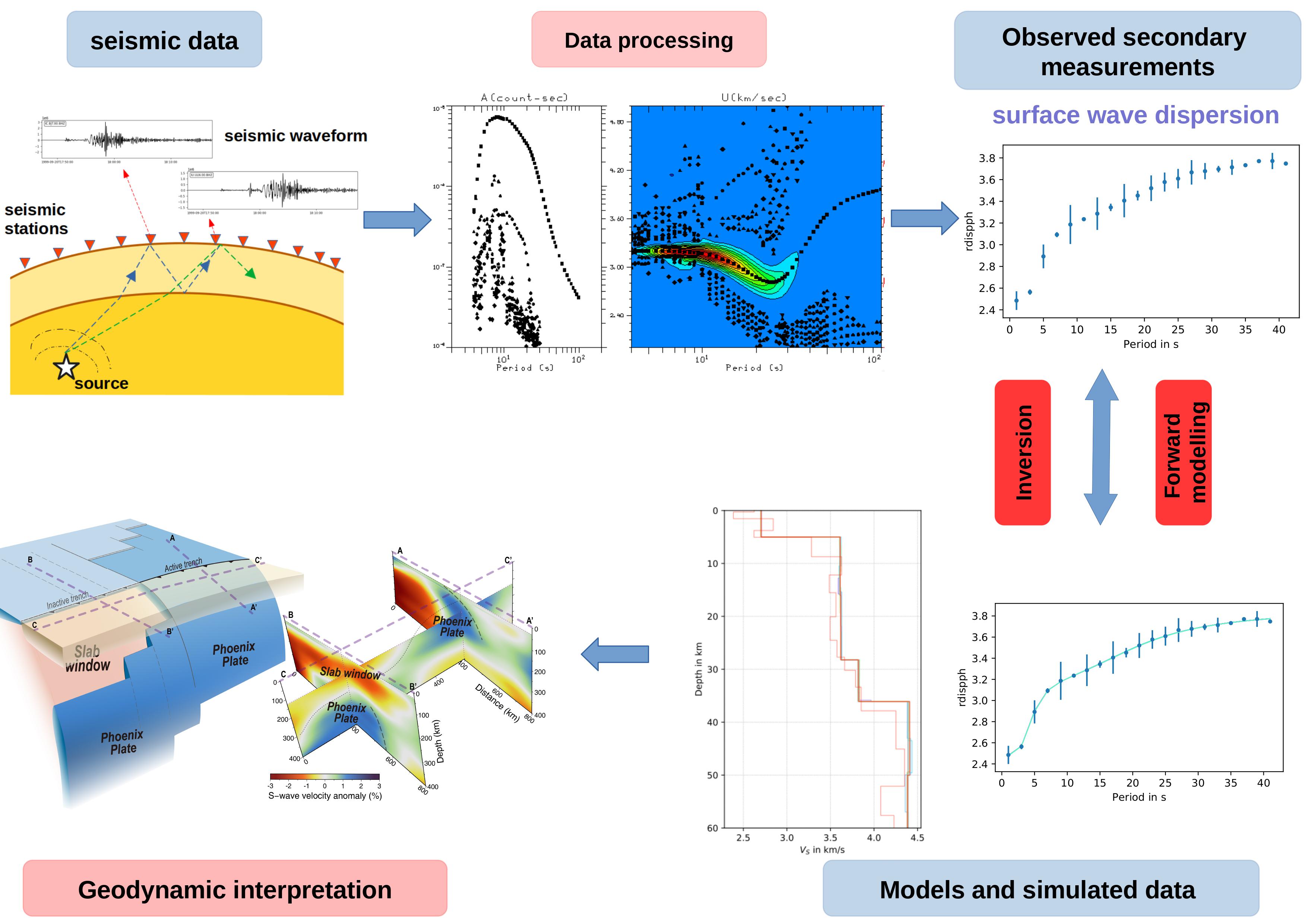
Fig. 81 A simple workflow shows the idea of seismic tomography. (Bottom left) The illustration of the shear velocity (Vs) anomaly model (right) and subsurface structure (left) is modified from [Li et al., 2021] .#
Sources of Uncertainty#
In seismic tomography, seismic data are acquired, processed, analysed, modelled, and interpreted in order to generate knowledge of the Earth’s interior where each processing step is affected by a certain degree of uncertainty related to the data and models and accumulate to the total uncertainties of the outputs. Here we introduce the sources of uncertainty from surface wave tomography.
Data-induced uncertainty:
Measurements errors of surface wave dispersion: frequency of outliers, correlated noise, noise-induced measurement uncertainties, and unknown errors. This refers to uncertainties in measuring the properties of surface waves, such as their velocity or dispersion characteristics. For example, instruments used to measure dispersion may have inherent errors, which can lead to inaccuracies in the data. Imagine using seismometers to measure the arrival times of surface waves; variations in the instrument’s sensitivity or calibration can introduce measurement errors
Geometry: the positioning and uneven distribution of sources and receivers can introduce uncertainty (see Fig. 82 ). For instance, if seismic sources and receivers are not evenly spaced or are located in regions with varying geological features, it can affect the quality of the data. Uneven distribution can lead to under-sampling in certain areas, making it challenging to accurately resolve subsurface structures.
Method-induced uncertainty:
Processing errors: parameter choices and subjective operations, for example, when manually picking dispersion curves from recorded data, there’s a potential for subjectivity and human error.
Forward model uncertainty: the mathematical model or the forward theory-based errors (physical approximation) to calculate surface wave dispersion. These models are simplifications of complex physical processes, and deviations from reality can introduce uncertainty. For example, a simplification in the model that assumes a homogeneous subsurface when it’s actually heterogeneous can lead to model inaccuracies.
Non-uniqueness in the model: geophysical inversion often encounters the problem of non-uniqueness, where multiple subsurface models can fit the observed data equally well. This means that there are multiple plausible solutions, and the true subsurface structure may not be uniquely determined.
Inversion algorithms: the choice of inversion algorithm and its parameters can affect the final result. For instance, regularization parameters used in linearized inversion methods can influence the level of smoothing applied to the model. In Bayesian inference, insufficient sampling or convergence can lead to uncertainties in the estimated posterior distributions.
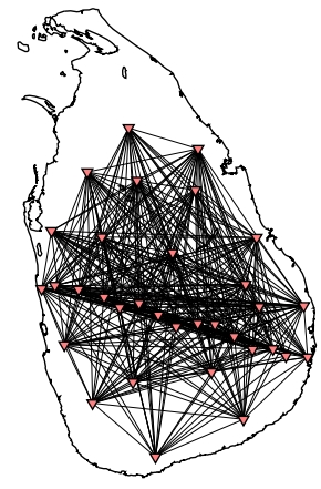
Fig. 82 Ray path coverage example to show that the uneven distribution on sources and receivers causes some regions to have poor ray coverage.#
Method: Hierarchical Transdimensional Bayesian Approach#
Conventionally, seismic inversion is treated as an optimization problem and proceeds through a linearized approach. In optimization problems, since most inverse problems are ill-posed, an optimal regularization parameter is selected to to make the optimal solution unique. However, these non-data-driven constraints (regularization parameter) on the model may cover essential information provided by the data and then underestimate data uncertainties. Furthermore, the resulting single best model given by an optimal regularization parameter reduces the number of possible models and lacks the capability to estimate model uncertainties.
To avoid regularization parametrization and quantify uncertainty a hierarchical transdimensional Bayesian framework, where data noise and the number of dimensions are viewed as unknown, has been applied in many geoscience studies. The approach takes non-uniqueness into account thus enables us to retrieve a large number of representative models which all fit the measurements very well. In addition, by treating data noise and model dimension as unknowns, data itself can decide the degree of fit and model complexity that is required.
References#
- LYH+21
Wei Li, Xiaohui Yuan, Benjamin Heit, Mechita C Schmidt-Aursch, Javier Almendros, Wolfram H Geissler, and Yun Chen. Back-arc extension of the central bransfield basin induced by ridge–trench collision: implications from ambient noise tomography and stress field inversion. Geophysical Research Letters, 48(21):e2021GL095032, 2021.
Contributors#
Nabir Mamnun, Frederik Tilmann