Species Abundance Distribution: Multivariate Approaches

Unlike the parametric and non-parametric approaches, the goal of the multivariate approach is typically to quantify and understand compositional variation between communities, termed beta diversity. A number of methods fall under the multivariate approach. First, various clustering methods may be used to classify communities into different types. Second, dimensionality reduction methods may be used to derive lower-dimensional representations of compositional data and order communities along major axes of variation. These axes are usually interpreted as environmental gradients important in shaping community composition. Because they order sites along important dimensions of variation, these dimensionality reduction methods are usually termed ordination methods in ecology. Common ordination methods used in ecology include principle components analysis (PCA), principle coordinates analysis (PCoA), and non-metric multidimensional scaling (NMDS). See [Manly and Alberto, 2016] for a good overview of these methods.

When considering ordination methods, a further distinction can be made between those that are computed directly on the matrix of species (relative) abundances and those that are computed on a matrix of pairwise dissimilarities between all sites.

Here we will focus on multivariate methods of analysis that use pairwise dissimilarities as their input. We will begin by illustrating the connection between measures of compositional dissimilarity and beta diversity. We will then introduce a common measure of compositional dissimilarity. Finally, we will give a short example of a multivariate analysis of multiple communities based on compositional dissimilarity.

Beta Diversity and Compositional Dissimilarity

When comparing multiple communities, diversity can be partitioned into multiple components. For example, consider a region that contains two sites (communities) where all species have been recorded. We will use species richness as our measure of diversity. We can partition the diversity of this region into three components, alpha (\(\alpha\)), beta (\(\beta\)), and gamma (\(\gamma\)) diversity. Alpha diversity is the average diversity of a single site, gamma diversity is the diversity of the entire region, and beta diversity is the average diversity between sites. For now, we will define the relationship between these diversities as additive such that

\[ \alpha + \beta = \gamma \]

Assume we counted 10 species at site A and 10 species at site B. If both sites have exactly the same set of species, then \(\alpha = 10\), \(\beta = 0\) and \(\gamma = 10\). If both sites have completely different species, then \(\alpha = 10\), \(\beta = 10\), and \(\gamma = 20\). This example illustrates that beta diversity can be thought of as the compositional dissimilarity between sites. If compositional dissimilarity between sites is high, then beta diversity is high. If compositional dissimilarity between communities is low, then beta diversity is low. Measures of compositional dissimilarity can therefore be used as measures of beta diversity.

Measures of Dissimilarity

To calculate compositional dissimilarity, the vectors of species abundances (or relative abundances) at two or more sites are considered as points in multivariate space and some measure of pairwise (dis)similarity is calculated between them. Measures of ecologically meaningful measures of dissimilarity are usually formulated in terms of species overlap between communities. Moreover, these measures are usually bounded between 0 and 1. For example, if two communities have the same species in exactly the same abundances, the compositional dissimilarity between them is 0. If two communities share no species in common, compositional dissimilarity takes a maximum value of 1. A common measure of compositional dissimilarity is the Horn dissimilarity or Horn distance [Horn, 1966] between sites \(i\) and \(j\).

Starting with an \(M \times N\) matrix \(A\) where \(M\) is the number of sampled sites and \(N\) is the number of species across all sites and each entry \(A_{ij}\) is the relative abundance of species \(i\) at site \(j\), we obtain an \(M \times M\) matrix \(D\) where each entry is the Horn dissimilarity between sites \(i\) and \(j\)

(17)\[ D_{ij} = 1 - \frac{\sum_n{(A_{in} + A_{jn})\ln(A_{in} + A_{jn})} - \sum_n{A_{in} \ln(A_{in})} - \sum_n{A_{jn} \ln(A_{jn})}}{2\ln(2) - 2\ln(1)}. \]

Example

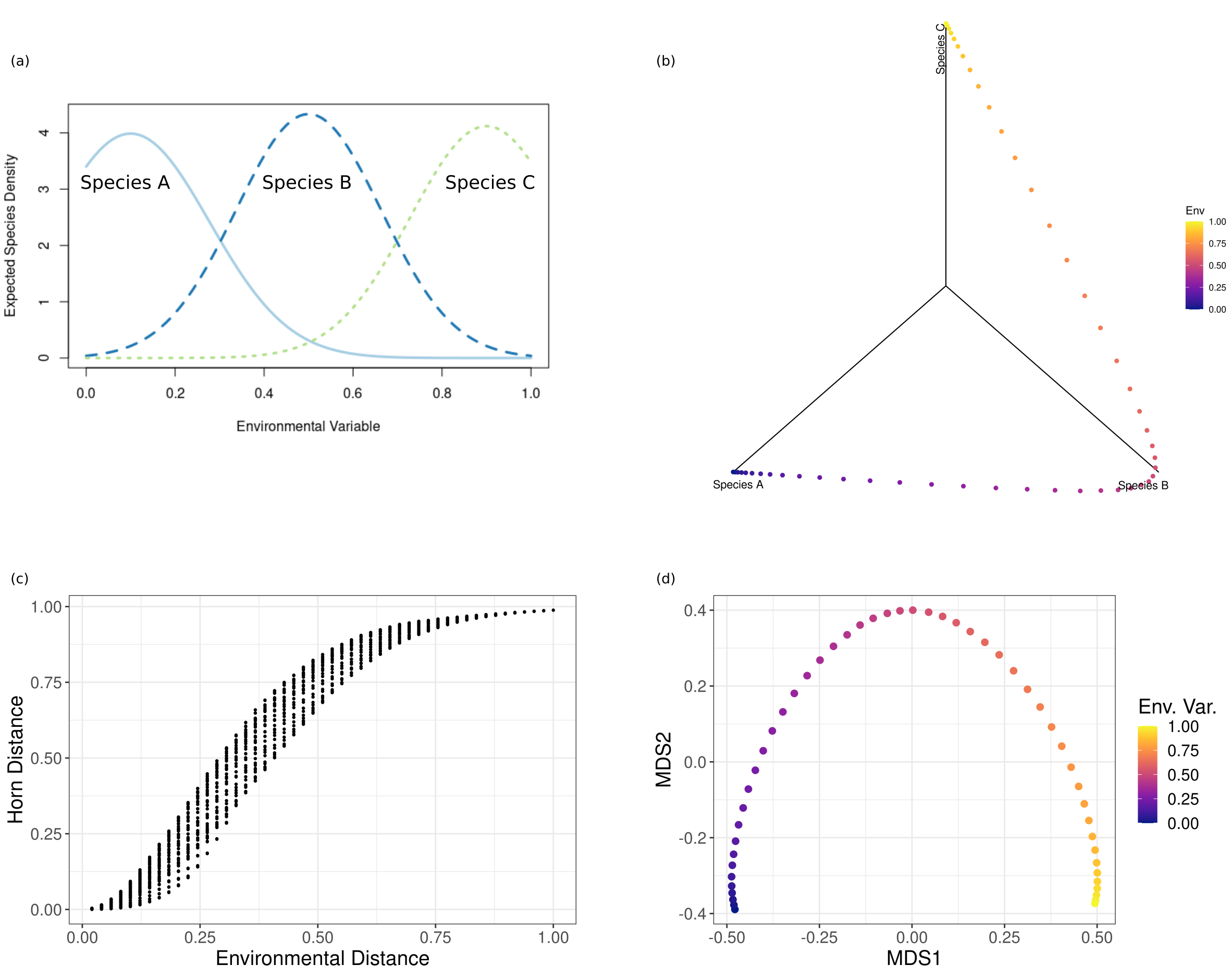
Fig. 71 Multivariate analysis of artificial species assemblages. a) Response curves for three species to a single environmental gradient. Each curve defines the expected number of individuals sampled at a given value of the environmental gradient. b) Plot of the relative abundance of the three species at 50 locations along the environmental gradient. Abundances were obtained as Poisson variates with expectation values defined by the response curves. Points are shaded by their location along the environmental gradient. c) Plotting pairwise compositional dissimilarities against environmental distance indicates that compositional dissimilarity increases along the environmental gradient. d) NMDS finds a lower-dimensional representation of the compositional data.

Two distinct but closely related approaches can be taken to understand how beta diversity is related to environmental and spatial gradients [Tuomisto and Ruokolainen, 2006]. First, we might wish to know how dissimilar two communities will be based on how environmentally dissimilar or geographically distant they are (i.e. how much compositional change can we expect for a given change in environmental conditions or geographic distance). Second, we might wish to know how community composition changes in response to environmental factors or geographical location (i.e. will a community have a specific composition for a specific set of environmental values or at a specific location). Using artificial species assemblages, we present below a short example of two common multivariate approaches used to address these questions.

If we sample species abundances at multiple sites, the compositional data from each site is a vector of species abundances (or proportional abundances). Each site can therefore be considered a point in multivariate space where each dimension corresponds to the abundance of a single species. Comparing the sites requires calculating the distance between points in this multivariate space.

For example, consider a simple case where three species exhibit a uni-modal response to a single environmental gradient (Fig. 71a). Sampling species at sites along the gradient and plotting the resulting abundances yields a three-dimensional curve (Fig. 71b). We begin by calculating all pairwise distances between points along this curve, obtaining a matrix of pairwise distances between the sampled sites. We use the Horn distance (17) as our measure of distance.

We can also calculate the distance between all pairs of sites along the environmental gradient, obtaining a matrix of pairwise environmental distances between the sampled sites. We can then plot the pairwise compositional distances against the pairwise environmental distances (Fig. 71c) to see that compositional dissimilarity increases as the environmental distance between sites increases. A common analysis is to use these pairwise compositional dissimilarities as the response variable for regression analysis with the aim of predicting the expected amount of compositional change for a given change in environmental conditions or geographic distance.

When seeking to understand how community composition changes in response to environmental factors or geographical location, it is often desirable to reduce the dimensionality of the data, summarizing the main features of community composition in a reduced number of variables. A common method of dimensionality reduction used in ecology is non-metric multidimensional scaling (NMDS). NMDS seeks a lower-dimensional configuration of the data in which the rank order of pairwise distances is as close as possible to the original dissimilarity matrix. Applying NMDS to the data plotted in (Fig. 71b), we can plot the curve in a lower-dimensional configuration space (Fig. 71d). We have chosen a two-dimensional configuration to illustrate that NMDS seeks to preserve the multivariate structure of the data in lower dimensions, in this case preserving the curvature of the data. In reality, the community composition is structured by a single environmental gradient, and we see that sites are ordered along this gradient along the first NMDS axis (Fig. 71d). The position along the first NMDS axis could thus be used as a univariate description of community composition which can in turn be used to model changes in community composition in response to environmental and spatial variation.

As the structure of multivariate compositional data becomes more complex, measures of pairwise dissimilarity become subject to bias and error, leading to potentially major issues with the above analysis. See the diffusion map case study article for a description of these sources of bias and error and a method for dealing with them.

References

Hor66

Henry S Horn. Measurement of" overlap" in comparative ecological studies. The American Naturalist, 100(914):419–424, 1966.

MA16

Bryan FJ Manly and Jorge A Navarro Alberto. Multivariate statistical methods: a primer. Chapman and Hall/CRC, 2016.

TR06

Hanna Tuomisto and Kalle Ruokolainen. Analyzing or explaining beta diversity? understanding the targets of different methods of analysis. Ecology, 87(11):2697–2708, 2006.

Authors

Jordan A. Gault