Measurement (DRAFT)#
Part of a series: Data-induced Uncertainties.
Follow reading here
This article is under construction.
Introduction#
We collect and analyze data in order to understand mechanisms which should provide a solid foundation for decisions to be made. Therefore, no analysis is funded just for fun, but is rather focused on the alternatives at hand and constantly compared with other results. Thus, the value of data lies in its power to produce reliable and replicable insights. Both of these are affected by measurement uncertainty which refers to the inability or doubt to observe data about a quantity of interest, the measurand \(M^{true}\), perfectly. Strictly speaking, we are making errors during the measurement process and hence cannot be certain to what degree some variable in our data set, \(M^{measured}\), reflects the actual value of an individual or patient.
The fields of physics and chemistry transcribed definitions and approaches to quantify the impact of this uncertainty during the 90’s in the so-called Guide to the Expression of Uncertainty in Measurement (GUM). In this guide, measurement uncertainty is defined as a “parameter, associated with the result of a measurement, that characterizes the dispersion of the values that could reasonably be attributed to the measurand” [Willink, 2013]. By now, even ISO-standards (no. 5725 and 17025 emerged, dealing with terms to describe the accuracy of measurement methods and stating requirements for the reporting.
The experimental nature of those disciplines enables them to adjust conditions and quantify the sensitivity of subsequent analyses accordingly. This, however, is not always possible. Observational studies often can neither manipulate such external factors nor repeat the measurements. Dealing with measurement uncertainty is particularly difficult in these settings.
Overall, understanding these issues and ways to account for them, can improve reliability of your models and conclusions you draw from them.
Variants of Measurement Uncertainty#
In general, the relationship between the true and the measured quantity can take any functional form \(M^{\mathrm{measured}} = f(M^{\mathrm{true}})\). In practice, however, the total error is often assumed to be additive and expressed as a sum of two components: a systematic error \(\beta\) and a random (individual) error \(\epsilon_i\) for the \(i\)-th observation.
The graphic below serves as an (admittedly somewhat artificial) example for measurement uncertainty. Here, \(y\) is the observable variable and takes a functional form of its true but latent counterpart \(x\) (sampled uniformly from the interval \([0,10]\)) and the specific measurement errors \(\epsilon\) and \(\beta\). How the error terms affect the relationship of this particular \(x\) and \(y\) is discussed throughout this section. This will highlight that knowing which component is present in your data may help to treat and report measurement uncertainty more accurately.
If, for instance, no systematic error is present (\(\beta=0\)) then the measurand is unbiased, i.e. \(\mathbb{E}(M^{\mathrm{measured}}) = M^{\mathrm{true}}\). Here, the measurement uncertainty can be treated as aleatoric and the uncertainty is negligible as it represents pure stochastic fluctuations around the true value. The green points and kernel density estimation in the graphic below show this scenario. The smoothed curve and the true data generating process in black are remarkably close. Nevertheless, this dispersion affects all further analyses. If \(M^{\mathrm{measured}}\) is used as a feature in a linear regression, the measurement uncertainty may yield increased residual errors, wider confidence intervals and thus a weaker correlation. The red points and smoothed line in the graphic indicate how larger \(\epsilon\)’s lead to wider confidence bands. Moreover large measurement errors can become outliers in a modelling approach and lead to implausible (in terms of unexpected) relationships. The challenge is to tell outliers and new phenomena apart. Mostly fixed thresholds (e.g. based on quantiles) are applied to identify outliers, but more sophisticated dynamic approaches have also been established [Tilmann et al., 2020].
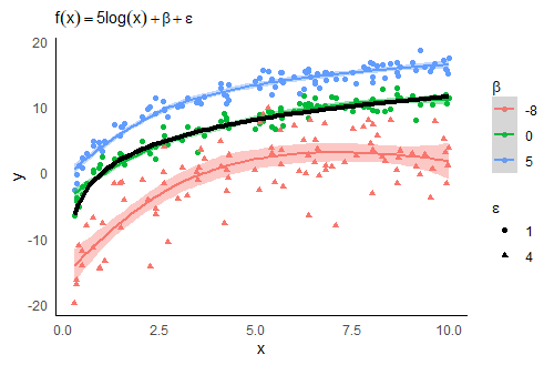
Fig. 16 Impact of random (\(\epsilon\)) and systematic (\(\beta\)) errors on kernel density estimations.#
The (more severe) second scenario includes epistemic uncertainty and produces the so-called measurement error/bias, i.e. \(\mathbb{E}(M^{\mathrm{measured}}) = M^{\mathrm{true}} + \beta\). Strictly speaking, the measured variable differs systematically from the true one and represents (without further considerations) a poor proxy for the variable of interest in subsequent analyses. This scenario is highlighted by both, the blue and the red coloured, configurations.
Dealing with Measurement Uncertainty#
The determination of measurement uncertainty prototypically consists of the following four steps:
Specify measurand
Identify & quantify uncertainty sources
Calculate combined uncertainty
This is often carried out in one of two approaches:
Top-down
Bottom-up
Top-Down approach#
The top-down procedure quantifies the measurement uncertainty by replication. This means a whole experiment is repeated, or observations are collected several times and the results are compared afterwards. This provides information about intra-laboratory repeatability and inter-laboratory reproducibility. The former one can be maximized (which is then called intermediate precision) by spreading trials over different days, using various machines, temperatures, etc. In general, the impact of external factors is marginalized and serves as a proxy for these kind of (technical) limitations. When several laboratories are involved the inter-laboratory reproducibility increases due to discrepancies in calibrations and different working styles (special form of observer bias).
Bottom-Up approach#
The bottom-up approach defines the overall uncertainty as a function of independent subsequent steps, such as weighing, pipetting or filtration, during an experiment. It may help to visualize the experimental set-up as a flow or think about the measurement as a composition of various elements. Then, imagine that the error traverses through each part of the process (called error propagation). Suppose that the final outcome of an experiment, \(M= f(x_1,\dots,x_n)\), consists of the quantities \(x_1,x_2,\dots,x_n\) (e.g. from intermediate steps). If \(u(x)\) denotes the added uncertainty from the source \(x\), then the overall uncertainty becomes
Conceptually, the formula above represents a weighted sum of the individual variances with the impact of each component expressed as partial derivative. Hence, one often says that “independent uncertainties add up quadratically” [Berendsen, 2011]. Please note that \(u(M)\) is derived from a Taylor expansion in which higher order terms were neglected. Thus reasonable small magnitudes for all \(u(x_i)\) neighbourhoods are assumed as well as their independence [Hughes and Hase, 2010]. If the components \(x_i\) are actually interdependent, their covariance structure must be incorporated in \(u(M)\) which makes its form more complex.
If, on the other side, the functional form \(f\) is simple, the formula simplifies as the following examples display:
Nonetheless, the specific calculation might be tedious in general and cannot be applied at all without an explicit mathematical model. In such scenarios, Monte Carlo based methods may be used instead. Here, input values \(\mathbf{x}^{(i)} = (x_{1}^{(i)},\dots, x_{n}^{(i)})\) are iteratively drawn either from a certain distribution or nonparametrically (e.g. using bootstrap) which are then used to derive estimates \(\hat u(\mathbf{x}^{(i)})\).
The fourth and last step finally yields the expanded uncertainty. The standard uncertainties \(u(x_i)\) are not necessarily standard deviations, but simply the contributions of uncertainty components. For most distributional forms \(u(M)\) covers a range between \(55\) and \(65\)% of the expected data. However, we are mostly interested in \(95\)% intervals and hence need to inflate this value appropriately. In practice, \(u(M)\) is multiplied by the corresponding quantile from the assumed underlying distribution. The QUAM guide for quantitative chemical analyses mentions the uniform distribution (when little is known about the function), the triangular form (when the measurement is concentrated around the middle) and the normal distribution which then yields \(u_{0.95}(M) = z_{0.95}\cdot u(M)\approx 2 u(M)\) [Group et al., 2000].
Masurement Uncertainty in scRNA-Seq Experiments#
Microbiological experiments provide good examples to highlight measurement uncertainty because quantities of interests are rarely observable (e.g. concentration of bacteria or molecules), but measured by proxies. For instance, an important goal of analyzing RNA samples is to distinguish groups of biological cells in terms of their gene expression levels (the proportion of molecules that belong to a certain gene). In practice, one cannot observe and count these molecules directly. Instead, several intermediary steps are necessary to cut the molecules, enrich the sample and visualize each nucleic base. The final output are millions of shorter duplicated RNA sequences which are supposed to appear proportional to the original RNA sample. How such a sample reacts to each of the sequencing steps might depend on external factors like temperature, waiting times and pressure. Hence, the outcome might vary even for identical samples! The Top down approach would recommend to repeat the experiments under numerous conditions and to report the dispersion.
Moreover, each laboratory assistant has his/her individual working style and thus adds another level of fluctuation. Let the same person analyze all samples may help to minimize this observer bias and hence increases consistency across measurements.
Regardless of all that, each sample has exactly one true value for its expressed genes, which is hopefully, but not necessarily related to our measurements. We should keep this uncertainty in mind when we draw conclusions and publish results. Finally, reporting MU in a standardized way (such as the mentioned ISO norms) improves comparability and reliability of your analyses.
References#
- Ber11
Herman JC Berendsen. A student's guide to data and error analysis. Cambridge University Press, 2011.
- GWE+00
Eurachem/CITAC Working Group, Alexander Williams, SLR Ellison, M Rosslein, and others. Quantifying uncertainty in analytical measurement. Eurachem, 2000.
- HH10
Ifan Hughes and Thomas Hase. Measurements and their uncertainties: a practical guide to modern error analysis. OUP Oxford, 2010.
- TSM20
F. J. Tilmann, H. Sadeghisorkhani, and A. Mauerberger. Another look at the treatment of data uncertainty in Markov chain Monte Carlo inversion and other probabilistic methods. Geophysical Journal International, 222(1):388–405, 2020. doi:10.1093/GJI/GGAA168.
- Wil13
Robin Willink. Guide to the Expression of Uncertainty in Measurement. In Measurement Uncertainty and Probability, pages 237–244. 2013. URL: http://chapon.arnaud.free.fr/documents/resources/stat/GUM.pdf, doi:10.1017/cbo9781139135085.018.