Quantifying Uncertainty for Data Imputation Methods#
Imputation methods comprise a particular approach to deal with missing data. All of these methods have in common that they replace a missing item by one imputed value (single imputation methods) or by more than one value (multiple imputation). Hence, these methods are widely used to generate complete data sets that can be used for the original analysis. However, the imputed data are subsequently treated as real observed quantities. Complete data analysis may then yield biased parameter estimates or biased standard errors within statistical analyses. This is particularly a pitfall of single imputation methods whereas multiple imputation accounts for imputation uncertainty facilitated by imputing several different values. In addition to that, the performance heavily depends on the assumed missing data mechanism.
This article presents single and multiple data imputation as methods to complete data sets with missing values. Moreover, related methods to characterise induced uncertainty are described. More detailed discussions, however, are given in [Enders, 2010, Little and Rubin, 2002, Molenberghs et al., 2015].
The concepts of this article are illustrated with an artificial example provided in [Enders, 2010]. A company asks prospective employees to complete an IQ test. Applicants who achieve good results are hired by the company. After a probation period, a supervisor then assesses their job performance. Fig. 38 shows the relationship of IQ and job performance of hired employees. Applicants with IQ below 99 were not hired and their potential job performance not measured. Thus, the type of missing data can be regarded as missing at random (MAR).
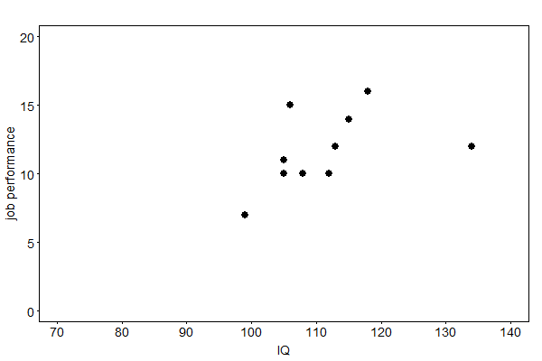
Fig. 38 The relationship of IQ and job performance of newly hired employees of a company#
Single Imputation Methods#
Single imputation methods generate one value for each missing data point. Though this approach might entail statistical shortcomings, some well known techniques are sketched.
Arithmetic Mean Imputation#
This method fills in the missing values of a variable with the arithmetic mean of the recorded values. Even though it is a convenient method, resulting parameter estimates may have a “large” bias, even in the missing completely at random (MCAR) setting. That is why mean imputation is sometimes regarded as “the worst missing data handling method available” [Enders, 2010], p. 43. The results of this method to the job performance example is depicted in Fig. 39.
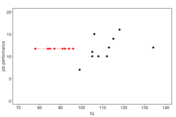
Fig. 39 Imputed job performances (red) by arithmetic mean imputation#
Hot-Deck Imputation#
Hot-deck imputation refers to methods that replace missing values by values from “similar” respondents in the sample. The statistical properties of the resulting estimates depend on the particular technique. On the one hand, some methods retain the variability of the imputed data. But on the other hand, unbiased estimates may only be derived for MCAR data.
Regression Imputation#
Another approach to fill in data for a variable with partially missing values is to compute a regression of the variable on other variables based on the complete cases. The corresponding regression equation is then used to predict the missing values. If more than one variable exhibits missing data, an individual regression equation needs to be derived for each variable. Fig. 40 shows imputed data for the missing job performances of not hired applicants.
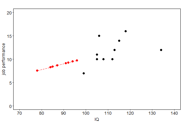
Fig. 40 Imputed job performances (red) by regression imputation#
Although regression imputation may come along with better statistical properties than mean imputation, it may still yield biased estimates. Due to the lack of variability of the imputed data, sample variances and covariances are in general attenuated.
Stochastic Regression Imputation#
The principle of stochastic regression imputation is similar to regression imputation. However, it induces more desirable properties for subsequent statistical analyses by adding random fluctuations to the predictions.
In order to illustrate the method, we assume that a data set contains \(n\in\mathbb{N}\) different subjects with \(p\in\mathbb{N}\) characteristics. Further, we assume that variable \(Y_p\) is only observed for the first \(r<n,~r\in\mathbb{N},\) subjects whereas \(Y_1,\dots,Y_{p-1}\) are fully observed for all \(n\). For sake of simplicity, we assume that \(Y_p\) linearly depends on \(Y_1,\dots,Y_{p-1}\). It allows us to compute a standard linear regression of \(Y_p\) on \(Y_1,\dots,Y_{p-1}\) based on the complete observations yielding the regression coefficients \(\beta_0,\dots,\beta_{p-1}.\) In comparison to regression imputation, a normally distributed random variable is added to the predictions calculated by the regression equation in order to obtain the imputed values. Formally, the imputed values are conditional draws according to
where the \(z_i\)’s are normally distributed random variables with zero mean and a variance equal to the residual variance of the regression. A graphical illustration of this method for the example of job performances is given in Fig. 41.
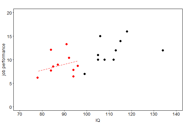
Fig. 41 Imputed job performances (red) by stochastic regression imputation#
The additional residual term for the imputed scores improves the imputation procedure compared to other single imputation methods. Incorporating these random components preserves the variability of the data. As a result, this imputation method yields unbiased and consistent parameter estimates from the filled-in data under an MAR assumption. Hence, it stands out among all single imputation methods.
Nevertheless, this technique has a shortcoming. Since filled-in data are again treated as real values in a subsequent analysis, standard errors of parameter estimates are, in general, inappropriately small. The multiple imputation approach explicitly addresses this problem of imputation uncertainty.
Quantifying Uncertainty for Single Imputation Methods#
In this section, two resampling methods are presented to quantify uncertainty induced by single imputation. In general, explicit formulas for variance estimates of parameter values are not available. But resampling methods can be applied to overcome this problem and they are also broadly applicable. These methods consist of imputing different values for the resampled incomplete data in order to compute the variability of point estimates of parameters. To do so, one needs to assume that the applied imputation method has eliminated the bias due to missing values. Besides, it is assumed the original statistical analysis on the completed data set yields estimate(s) \(\hat{\theta}\) of the parameter(s) of interest \(\theta\). The resulting variance estimates can subsequently be used to construct confidence intervals.
Bootstrapping#
The bootstrapping approach starts with the generation of bootstrap samples \(S^{(b)},~b=1,\dots,B,\) from the original unimputed data set \(S\) of \(n\) observations. Using some single imputation method on every sample \(S^{(b)}\) yields the filled-in samples \(\hat{S}^{(b)},~b=1,\dots,B.\) Then, the parameter estimates \(\hat{\theta}^{(b)},~b=1,\dots,B,\) can be computed for every \(\hat{S}^{(b)}.\) The bootstrap estimate is defined by
The bootstrap estimate of the variance,
is a consistent estimate of the variance of \(\hat{\theta}.\)
Jackknife Resampling#
Again, the original data set is denoted by \(S\) with \(i=1,\dots,n\) observations some of which exhibit missing variables. For every \(i\), \(S^{(\setminus i)}\) denotes a sample of size \(n-1\) which is identical to \(S\) only without observation \(i\). The missing values of \(S^{(\setminus i)}\) are filled in with a chosen imputation technique yielding the complete sample \(\hat{S}^{(\setminus i)}.\) The corresponding parameter estimate(s) is (are) denoted by \(\hat{\theta}^{(\setminus i)}.\) For \(\tilde{\theta}_i=n\hat{\theta}-(n-1)\hat{\theta}^{(\setminus i)}\), the jackknife estimate is then given by
The jackknife estimate of the variance can be written as
where
\(\hat{V}_{jack}\) is a consistent estimator of the variance of \(\hat{\theta}.\)
Multiple Imputation#
In contrast to single imputation methods, multiple imputation creates several copies of an incomplete data set imputed with different values for each missing data point. This approach accounts for the uncertainty inherent in the imputation of missing values. Along with likelihood-based approaches, multiple imputation is sometimes referred to as one of the “state-of-the-art” imputation methods [Enders, 2010], p. 187. This method assumes that the missing data follows an MAR mechanism.
Conceptually, it mainly consists of three different phases; the “imputation phase”, the “analysis phase” and the “pooling phase”. We are going to describe each phase separately. In order to do so, we adopt the formal framework from the previous section. An overview of the three different phases is shown in Fig. 42.
Imputation Phase#
The imputation phase can be regarded as the core of multiple imputation. Within this phase, it imputes different values for the missing data. This procedure is usually conducted in a Bayesian framework. In this connection, several imputation algorithms are available addressing different types of problems. The data augmentation (DA) algorithm is one of the most used algorithms. It is an iterative algorithm that alternately draws imputed values and updates parameter values. We denote its iterations by \(t=1,\dots,T\). Moreover, for a given data set \(Y\), we denote by \(Y^m\) and \(Y^o\) the missing portion and the observed portion, respectively, of the data. The (set of) parameter value(s) \(\theta^{(0)}\) characterizes the imputation in the first iteration. Each iteration \(t\) then consists of two steps:
I-Step: Draw imputed values from their conditional distributions, i.e. draw
\[ \begin{align*} Y^m(t)\sim p(Y^m|Y^o,\theta^{(t-1)}). \end{align*} \]P-Step: Update parameter values by drawing from the posterior distribution, i.e. draw
\[ \begin{align*} \theta^{(t)}\sim p(\theta|Y^o,Y^m{(t)}). \end{align*} \]
The imputation phase can be regarded as an iterative and generalized version of stochastic regression imputation. In terms of the illustration given for stochastic regression imputation (for \(p=2\)), the I-Step can be interpreted as drawing \(\hat{y}_{i,2}^{(t)}\sim\mathcal{N}(\beta_0^{(t-1)}+\beta_1^{(t-1)}y_{i,1},\sigma_{res}^{(t-1)})\) at iteration \(t\). The P-Step then consists of updating the parameters \(\beta_0^{(t)},~\beta_1^{(t)}\) and \(\sigma_{res}^{(t-1)}\) by recalculating the regression equation including the imputed values.
Furthermore, the DA algorithm is similar to the expectation-maximization (EM) algorithm which also consists of alternating iteration steps. But the main difference is that we draw updated parameters from the posterior distribution in the P-Step whereas the posterior (or likelihood function) is maximized in the maximization step (M-Step) of the EM algorithm.
In the limit, the draws in the two steps are taken from the joint posterior distribution of \(Y^m\) and \(\theta\). Thus, running the DA algorithm sufficiently long ensures that the draws are taken from the approximate joint posterior distribution of \(Y^m\) and \(\theta\). There are different methods available for assessing the convergence of the algorithm (e.g. graphical displays, like time-series plots or plots of the autocorrelation function). By repeating this procedure \(D\in\mathbb{N}\) times, we obtain \(D\) complete filled-in data sets. As a rule of thumb, it is common to generate at least \(D=20\) data sets.
Analysis Phase#
The analysis phase consists of performing the actual intended statistical analysis on the \(D\) filled-in data sets from the imputation phase. It yields \(D\) different (sets of) parameter estimates \(\hat{\theta}_t,\, t=1,\dots,D.\) These estimates are unbiased under an MAR mechanism.
Pooling Phase#
The pooling phase aims to combine the \(D\) different parameter estimates into one (set of) single point estimate(s). If we assume that the parameter estimates are asymptotically normally distributed, the pooled estimate equals the arithmetic average, i.e. the multiple imputation point estimate is given by
If asymptotic normality is not satisfied, a transformation of the parameter estimates may be necessary before combining.
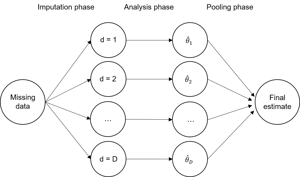
Fig. 42 The three phases of multiple imputation#
Quantifying Uncertainty for Multiple Imputation#
In this section, we present methods to quantify uncertainty of parameter estimates induced by multiple imputation. Basically, multiple imputation involves two sources of sampling fluctuation that enter standard errors. The impact of both sources can be calculated using quantities derived before.
The “within-imputation variance” estimates the sampling error that would have resulted if the data had been complete. It is defined by
i.e. the arithmetic average of the sampling variances (\(SE_t\) denotes the standard error from data set \(t\)).
Due to multiple imputation, we also need to account for the fluctuation of parameter estimates across the \(D\) data sets caused by the different imputed values. The so-called “between-imputation variance” is given by
where \(\hat{\theta}_t\), for \(t=1,\dots,D,\) and \(\bar{\theta}\) are again the single parameter estimates from the \(D\) data sets and the multiple imputation point estimate, respectively.
The “total sampling variance” is then defined as
Here, the term \(\frac{\hat{V}_B}{D}\) captures the sampling error of \(\bar{\theta}\) involved in \(\hat{V}_B\).
Based on these three quantities, the impact of missing data could be further investigated. For example, the “fraction of missing information” can be computed or confidence intervals can be constructed.
References#
- End10(1,2,3,4)
Craig K. Enders. Applied Missing Data Analysis. Guilford, 2010.
- LR02
Roderick J. A. Little and Donald B. Rubin. Statistical analysis with missing data. John Wiley & Sons, Inc, 2002.
- MFK+15
Geert Molenberghs, Garrett Fitzmaurice, Michael G. Kenward, Anastasios Tsiatis, and Geert Verbeke. Handbook of Missing Data Methodology. CRC Press, 2015.
Contributors#
Jonas Bauer