Stochastic Inference in Load-Frequency Control

Part of a series: Uncertainty in Future Energy Systems.

Follow reading here

The transformation of the energy system towards CO\(_2\) neutral generation is an essential measure to mitigate the effects of climate change. This energy transition is affecting the operation and stability of electric power systems on very different levels and in a complex manner. Conventional generation by mostly thermic power plants that rely on fossil fuels have to be replaced by by renewable sources (i.e., wind turbines and solar panels), which are volatile and inherently uncertain.

One challenge in power system operation is the control of the generation, which has to be matched to the load at all times. This control is essentially based on the grid frequency, whose dynamics provides comprehensive information about the system [Gorjão et al., 2020]. Since most large-scale electric power grids are run using alternating current, the current and voltage oscillate with a frequency, which is close to a nominal frequency, throughout the entire synchronous electricity grid. This power grid frequency changes due to power imbalances in supply and demand of electric power. The speed of this change and the frequency dynamics is determined by the inertia. Inertia is provided mostly by thermic generators that are synchronously coupled to the grid and thus slow down a potential change in grid frequency by supplying some rotational power of their large rotating generator masses.
Various control mechanisms are used to keep the grid frequency in acceptable operation margin around the nominal frequency \(\omega_0\) to restore the balance of generation and load. The two fastest and important ones are primary and secondary control. While primary control has to fully deploy the maximal amount of power in 30 seconds to limit a frequency deviation due to a disturbance, secondary control has a longer activation time of around 15 minutes and brings the system back to the nominal frequency. The grid frequency is also affected by noise that can originate from different sources with the most prominent one being random fluctuations in generation and load. Separating deterministic trends, unforseen large disturbances (e.g., a transmission line failing) and random noise, requires an appropriate detrending method and a careful analysis of the underlying stochastic process.
In summary, the grid frequency encodes the complex state of the power system and thus represents an important observable to judge stability and condition of the power system.

Examining the stochastic features of the frequency dynamics by plotting a histogram of the observed frequency values reveals important features (see Fig. 56).

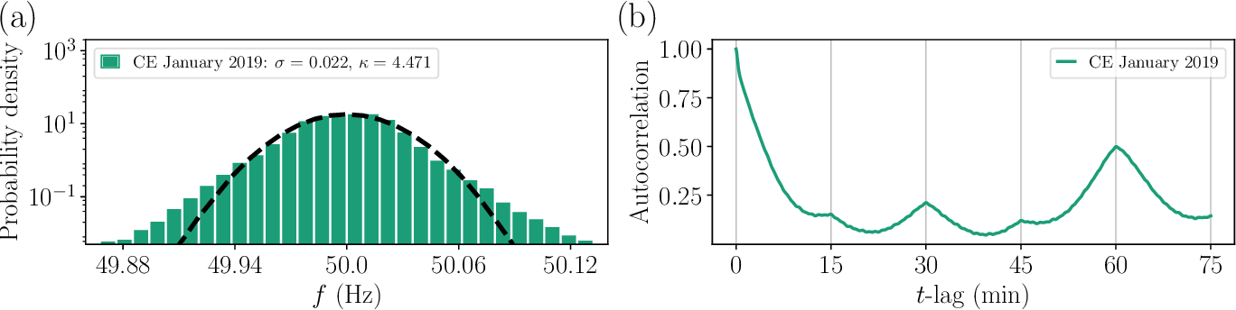
Fig. 56 The distribution of the power-grid frequency is heavy-tailed and and displays pronounced recurring patterns. (a) The histogram of the grid frequency displays heavy tails at both ends of the distributions that are not captured by a Gaussian distribution (dashed line), i.e., white noise. This is underlined by the high kurtosis \(\kappa\). (b) The autocorrelation function displays characteristic peaks every 15 minutes which appear due to the market activities of electricity markets. The frequency data was recorded by TransNetBW in January 2019. Figure is taken from [Gorjão et al., 2020] (CC BY 4.0).

The histogram shows heavy tails that cannot be explained by a Gaussian distribution and the auto-correlation function indicates that the fluctuations cannot be caused by simple time-independent white noise. Additionally, the autocorrelation displays prominent peaks every 15 minutes that can be explained by the current market design. Since electricity is traded in blocks of 15, 30 or 60 minutes, power generation is rapidly adjusted at the beginning of an interval and stays mostly constant in between. As the load changes continuously, the resulting imbalance has a saw-tooth shape with the highest imbalances at each end of a time interval (see Fig. 57). It is possible to describe the statistics of the considered time series by different approaches using, for example, non-Gaussian white noise, superstatistics or a suitable driving term.

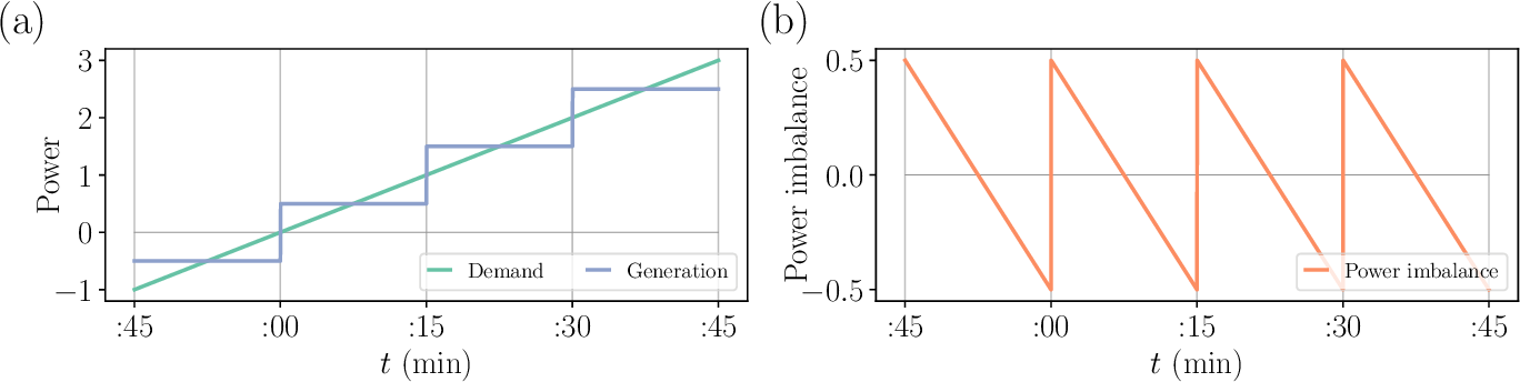
Fig. 57 (a) While generation is delivered with contracts that set a generation level for a certain amount of time (mainly 15 minutes and 1 hour), the demand changes continuously. (b) If one assumes a simple linear increase in demand, the resulting load imbalance is a saw tooth function with the highest power imbalances at each end of the time interval. While this example describes the principal features of market-based imbalances, it is worth mentioning that the demand does not change linearly in general but follows a distinctive daily pattern. Figure taken from [Gorjão et al., 2020] (CC BY 4.0).

A simple model that considers the aforementioned factors is the aggregated swing equation [Ulbig et al., 2014], which follows the stochastic differential equation given by

\[\begin{split} \begin{equation} \begin{aligned} \frac{d}{dt} \theta &= \omega \\ M \; \frac{d}{dt} \omega &= -c_1 \omega - c_2 \theta + \Delta P + \epsilon \xi \end{aligned} \end{equation} \end{split}\]

where \(\omega\) is the grid frequency, \(\theta\) is the power phase angle, \(M\) is the inertia, \(c_1\) is the coefficient of the primary control and other damping effects, \(c_2\) is the secondary control coefficient, \(\Delta P\) the power imbalance, \(\epsilon\) the noise strength, and \(\xi\) uncorrelated white noise. Note, this model closely resembles a harmonic oscillator with dissipation, thermal fluctuations and external forcing which represents a prototypical model in the study of dynamical systems.
In principle, this model regards the entire electricity system as one synchronous machine.

The SDE above is connected with a Fokker-Planck-Equation that describes the time evolution of the probability density \(p(\omega, t)\) of the system being in state \(\omega\) at time t. Assuming the deterministic trends are correctly captured by the proposed \(\Delta P\) and that contribution of secondary control are either small or removed from the trajectory by appropriately detrending, it reads

\[\begin{split} \begin{align} \frac{\partial p(\omega, t)}{\partial t} &= - \frac{\partial}{\omega} (-c_1 \; \omega \; p(\omega, t)) + \frac{\epsilon^2}{2} \frac{\partial^2 p(\omega, t)}{\partial \omega^2}\\ &= - \frac{\partial}{\partial \omega} \mathcal{D}^{(1)} \;p(\omega, t) + \frac{\partial^2}{\partial \omega^2} \mathcal{D}^{(2)} \;p(\omega, t) \end{align} \end{split}\]

where \(\mathcal{D}^{(1)}\) and \(\mathcal{D}^{(2)}\) describe the drift and diffusion, respectively. Here, the inertia \(M\) has been absorbed into each variable, since it only rescales the equation.

The drift and diffusion term can be estimated using Kramers-Moyal expansion [Gorjão and Meirinhos, 2019] from measured frequency data of Continental Europe, which enables us to obtain an estimate of the parameters \(c_1\), \(c_2\) and \(\epsilon\) assuming that a suitable estimate of \(\Delta P\) was chosen. Using a \(\Delta P\) motivated by the market induced imbalance (see Fig. 57) and determining a suitable size for the stepwise generation from data, reproduces the stochastic features of the grid frequency rather well (see Fig. 58).

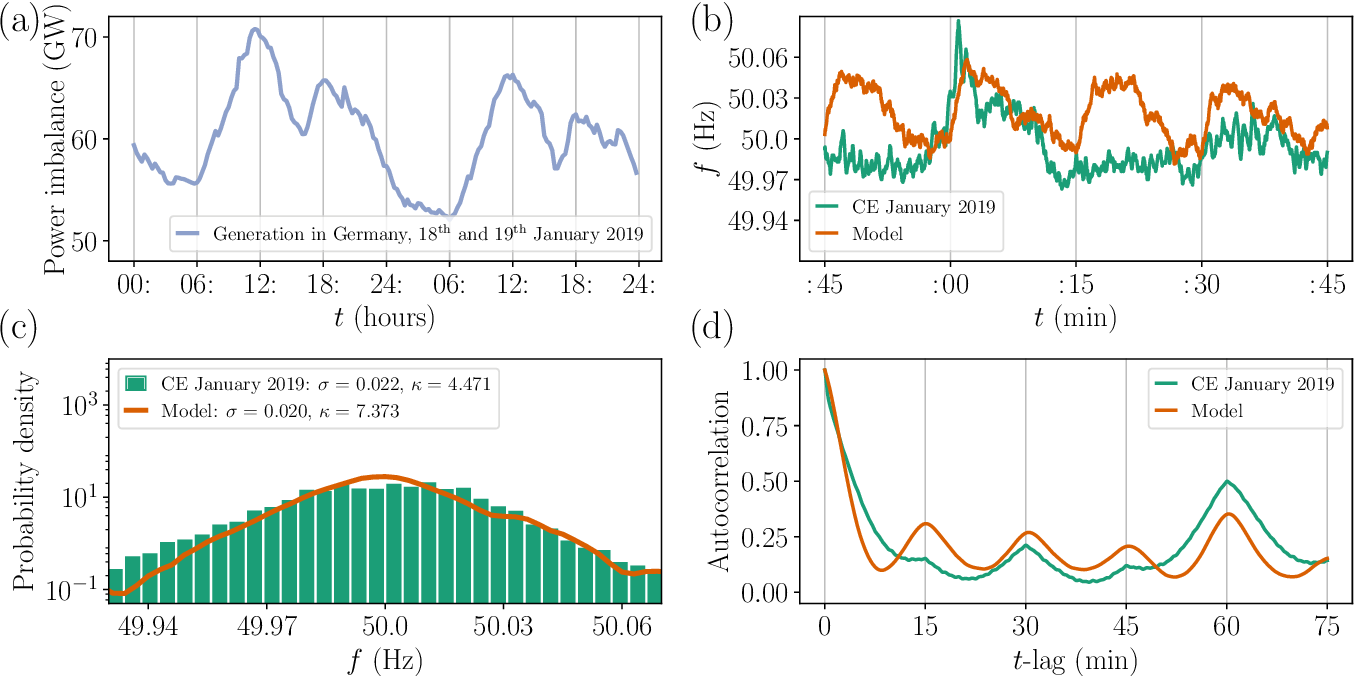
Fig. 58 Using a realistic dispatch in the stochastic model reproduces the essential statistic characteristics of measured frequency statistics. (a) Real power dispatch to obtain correct jumps of the Heaviside function. (b) Comparison of synthetic and measured frequency trajectory. (c) Histograms (d) The autocorrelation for a time windows of 75 minutes. Figure taken from [Gorjão et al., 2020] (CC BY 4.0).

In summary, this modelling approach bridges the gap between power engineering and stochastic modelling, which highlights how the frequency dynamics is influenced by market activity. Using this model can also be helpful when designing novel market designs, since it can be used to evaluate how different market designs might influence the frequency dynamics. A more detailed discussion of the model and the described stochastic features of the grid frequency can be found in [Gorjão et al., 2020].

References

GorjaoAK+20(1,2,3,4,5)

Leonardo Rydin Gorjão, Mehrnaz Anvari, Holger Kantz, Christian Beck, Dirk Witthaut, Marc Timme, and Benjamin Schäfer. Data-driven model of the power-grid frequency dynamics. IEEE access, 8:43082–43097, 2020.

GM19

Leonardo Rydin Gorjão and Francisco Meirinhos. Kramersmoyal: kramers–moyal coefficients for stochastic processes. Journal of Open Source Software, 4(44):1693, 2019. doi:10.21105/joss.01693.

UBA14

Andreas Ulbig, Theodor S Borsche, and Göran Andersson. Impact of low rotational inertia on power system stability and operation. IFAC Proceedings Volumes, 47(3):7290–7297, 2014.

Authors

Philipp Böttcher

Contributors

Sonja Germscheid, Dirk Witthaut