Bayesian Mixture Models

Introduction

Many disciplines deal with data that contains more than one single data generating process. Instead, population can often be further divided into subclasses which in turn may have distinct parameters. Sequencing data from biological cells, for instance, is quite likely to emerge from a mixture of classes due to cell heterogeneity. We might observe distinctive expression patterns for certain kind, age stages and stati of cells. Here, a class could represent whether a cell is healthy or diseased. Not only does the incorporation of classes reflect these biological characteristics and hence improves the model, but the membership information itself often is of great importance for researchers. Thus, this article describes mixture models in general, approaches for Bayesian inference as well as common obstacles along the way.

Mixture Models

The particular class of an individual \(i\) will be denoted by it’s latent class \(Z_i\). The class, in turn, determines the parameterization \(\beta^{(Z_i)}\) of the observed data \(C_i\). This means that given the class, the distributional form of a data point is known, i. e. \(C_i|Z_i \sim p(\beta^{(Z_i)})\). Nevertheless, the law of total probability allows us to still write the unconditional data distribution for \(K\) classes as follows:

\[ p(C) = \sum_{k=1}^K p(C|Z=k)\cdot p(Z=k) \]

The distribution of the latent classes may be described with their relative frequencies \(p(Z=k) = \pi_k \ \forall k\). Furthermore, the class-specific parameters are implicitly involved in the model above because the conditional data distributions depend on them. Overall, the parameters may be summarized as \(\theta = (\beta^{(0)}, \dots,\beta^{(K)},\pi_1,\dots, \pi_{K-1})^T\)

Estimation

To make estimation and sampling for mixture models more efficient Rubin and his colleagues included a completed data likelihood [Dempster et al., 1977]. This means we can extend an existing model to cover two states by incorporating the information as follows:

\[ p(\theta | C, Z) \propto \underbrace{p(C|\beta, Z)}_{\text{Completed}} \times \underbrace{p(Z|\pi)}_{\text{latent}} \]

Completed:

\[\begin{split} \begin{align} p(C|\theta, Z) &= \prod_{i=1}^{n} p(C_i|\theta, Z_i) = \prod_{k=1}^{K} \prod_{i|Z_i=k} \underbrace{p(C_i|\beta^{(k)}, Z_i=k)}_{= MN(\beta^{(k)})} \\ &\propto \prod_{k=1}^K \prod_{g=1}^G \left(\beta^{(k)}_g\right)^{\sum_{i|Z_i=k} C_i} \end{align} \end{split}\]

Formulae and implementations for the latent model become tedious1 when more than two classes are considered. Thus, we will focus on only two classes with \(Z_i\in \{0,1\} \ \forall i, \pi \in [0,1]\) here. The latent model can then be written as follows:

\[ \begin{align} p(Z|\pi)= \prod_{i=1}^n\pi^{Z_i}(1-\pi)^{1-Z_i}=\pi^{\sum_i Z_i}(1-\pi)^{n-\sum_i Z_i} \end{align} \]

A common frequentistic approach is to alternate multiple times between completion of the likelihood and its maximization with respect to the class-specific parameters which is then referred to as expectation-maximization algorithm. Here, the states are updated using so-called posterior responsibilities [Bishop and Nasrabadi, 2006]. This concept may be seen as simple Bayesian parameter updates. Before seeing any data, the probability to be from a certain class is the same for every observation and described by the initial guess \(\pi\). The data \(C_i\), however, provides additional information that should be taken into account. For instance, an a-priori unlikely class (\(\pi_k\) small) may have strong data support which increases the posterior responsibility. This is done by the following weighted average of class-specific conditional distributions:

\[ p(Z_i=k|C_i) = \frac{\pi_k p(C_i|Z_i=k)}{\sum_k \pi_k p(C_i|Z_i=k)} \]

Nevertheless, this article focuses on Bayesian inference instead for the following two reasons:

• We are interested in parameter uncertainty and hence aim to explore the whole posterior distribution.

• We are going to discuss extensions with variable number of classes \(K\) later.

An important part of Bayesian modelling deals with the form of prior parameter distributions. For two classes, the prior may be written as the following product:

\[ p(\theta) = p(\beta^{(0)}) \times p(\beta^{(1)}) \times p(\pi) \]

A typical choice for \(p(\pi)\) for any fixed finite \(K\) is a Dirichlet distribution. The posterior distribution of a Bayesian mixture model hence becomes the product of parameter priors, as well as latent and completed data distributions.

\[ p(\theta | C, Z) \propto \underbrace{p(C|\theta, Z)}_{\text{Completed}} \times \underbrace{p(Z|\pi)}_{\text{latent}} \times \underbrace{\prod_k p(\beta^{(k)}) \times p(\pi)}_{\text{priors}} \]

If the class-specific distributions are conjugate, parameter updates for \(\beta^{(k)}\) can be sampled directly from its posterior \(p(\beta^{(k)}|C,k)\). Please note, however, that the form of every class-specific posterior depends on the data points associated with this cluster. If the model is non-conjugate, costly MCMC parameter updates must be derived with some form of sampler like the Hamiltonian Monte Carlo algorithm. Thus, the computational effort and the choice of the algorithm depends on the model at hand.

Drawbacks

Mixture models can capture multi-modal densities and cluster distinct groups very well. On the contrary, two main drawbacks emerge:

1. Extended parameter space

2. Less robust to misspecification and/or bad initialization

If \(G\) denotes the parameter dimension for a single class, then the mixture parameter becomes a \((G\cdot K + K -1)\)-dimensional vector2. Apparently, there is no such thing as a free lunch. The greater flexibility of mixture models comes hand in hand with the curse of dimensionality. This is especially harmful when \(G\) is also large. Therefore, the estimation requires more space (larger matrices to be stored and potentially more iterations until convergence) and computational time. The computational effort increases because many samplers derive new proposals with linear complexity to the parameter dimension (e. g. Hamiltonian Monte Carlo requires the calculation of \(G\)-dimensional gradients). Hence, one should be careful when choosing the number of classes.

The second drawback is (at least partly) a result of the first. The more parameters are involved, the more starting values are required. These, in turn should be chosen adequately. Although any such chain should converge eventually, the time until this happens depends heavily on the distance to the actual high density regions. Also, one should keep in mind that an increased parameter space could contain more local optima. Finally, an additional parameter must be set: The number of classes. Choosing too few classes leads to the same lack of fit and “mixing classes together” that has led us to mixture models in the first place. Too many classes, on the other side, could lead to identifiability issues. Identifiability of a model means that a unique equilibrium exists. Hence, the markov chain that we sample from will eventually converge to this particular distribution. Fortunately, MCMC algorithms work in a fashion that guarantees this convergence as long as the model is well-defined. To illustrate this issue, we elaborate the behavior of a two-component mixture model without further restrictions fitted to a sample which indeed consists of two classes (\(K=2\)). Here, the first set of parameters \(\beta^{(0)}\) could model class 0 with the corresponding class probability of \(1-\pi\) or it could be used to fit class 1 with the counter-probability \(\pi\). For the model, it makes no difference whether we model \(p(C|Z) = \pi p(C|\beta^{(1)})+(1-\pi) p(C|\beta^{(0)})\) or flip the status for every observation and arrive at \(p(C|1-Z) = \pi p(C|\beta^{(0)})+(1-\pi) p(C|\beta^{(1)})\). In other words, with the latent status changed for every observation, we reach the exact same level of the objective function for every combination \((\beta^{(0)},\beta^{(1)}, \pi), (\beta^{(1)},\beta^{(0)}, 1-\pi)\). This particular issue can easily be solved by introducing the additional restriction \(\pi>1/2\).

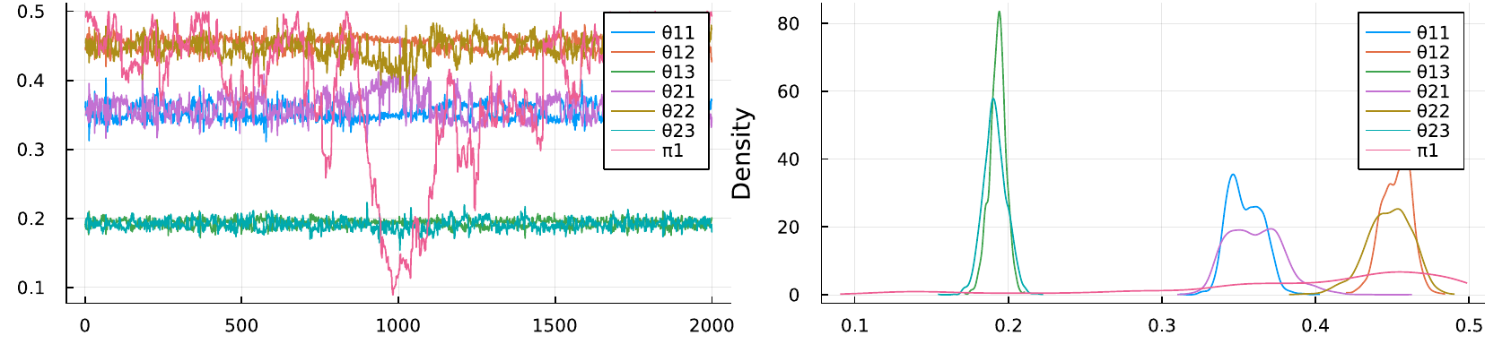
Fig. 31 Mixing (left) and kernel density (right) of posterior samples from a mixture model for which two classes were assumed, whereas the data was generated by only one class. Each class-specific distribution requires three parameters, i. e. \(\theta_{k,1},\theta_{k,2},\theta_{k,3}\).

Identifiability issues become more severe when we overestimate the number of classes. This means our model would be too complex and some parameters are not needed at all to model the data. The figure above shows the mixing of a two-class mixture model fitted to data from a single class. As can be seen, both class-specific sets of parameters render approximately the same densities. If both classes account for the same underlying population, then the mixing is irrelevant and the parameter can take any arbitrary value. This behaviour can be seen as furious exploration of the whole space for \(\pi_1\) in the left subplot and its flat density in the right subplot.

Extensions

Mixture models are certainly not a recent invention, but they are still used for latent multi-class problems with a decent amount of prior information regarding the number of classes. However, if \(K\) is a-priori not known, one can either sample from multiple mixture models using transdimensional MCMC or let the data decide whether another class is necessary in every MCMC iteration. The latter extension is called a Dirichlet process mixture model because a Dirichlet process is used for the mixing between a theoretically infinite amount of classes.

The flexibility gained with a Dirichlet process mixture model comes with the price of a more challenged estimation. To sample from such a posterior, various schemes have been developed. A good overview and tabularization can be found, for instance, in [Chang and Fisher III, 2013]. The three most important characteristics are as follows:

• Is the algorithm approximate (i. e. \(K\) truncated) or exact?

• Are the mixing weights marginalized or explicitly instantiated?

• Is the algorithm suited for conjugate or non-conjugate models?

[Li et al., 2019] provide a great tutorial for an exact sampler with marginalized weights for conditionally conjugate models based on the algorithm from [Neal, 2000]. The idea is to use the exchangeability of data points to reassign one point at a time using the following Gibbs update:

\[\begin{split} \Pr(Z_i=k|Z_{-i}, C_{-i}) = \begin{cases} \frac{n_{-i,k}}{N-1+\alpha} & \\ \frac{\alpha}{N-1+\alpha} & , k \neq Z_j \ \forall j \end{cases} \end{split}\]

This means we incorporate the information of all but the \(i\)-th assignment, \(Z_{-i}\), and their class-specific predictive distributions in order to find the next class of observation \(i\). This procedure, however, is inherently sequential and the computational effort is an order of magnitude of the sample size. This becomes particulary problematic in applications where continuous technological advances generate ever more data, such as high-throughput sequencing RNA from biological samples. One way out of this dilemma is to truncate the number of possible classes by a large natural number. Hence, the curse of dimensionality in scRNA data-article discusses this and other sampling approaches within the challenging field of single cell RNA analysis.

References

BN06

Christopher M Bishop and Nasser M Nasrabadi. Pattern recognition and machine learning. Volume 4. Springer, 2006.

CFI13

Jason Chang and John W Fisher III. Parallel sampling of dp mixture models using sub-cluster splits. Advances in Neural Information Processing Systems, 2013.

DLR77

Arthur P Dempster, Nan M Laird, and Donald B Rubin. Maximum likelihood from incomplete data via the em algorithm. Journal of the Royal Statistical Society: Series B (Methodological), 39(1):1–22, 1977.

LSGonen19

Yuelin Li, Elizabeth Schofield, and Mithat Gönen. A tutorial on dirichlet process mixture modeling. Journal of mathematical psychology, 91:128–144, 2019.

Nea00

Radford M Neal. Markov chain sampling methods for dirichlet process mixture models. Journal of computational and graphical statistics, 9(2):249–265, 2000.

Authors

Jonas Bauer

Contributors

Kainat Khowaja, Dirk Witthaut

---

1

For the interested reader: Using \(1_j(Z_i)=1 \iff Z_i = j \ , \ \pi \in [0,1]^K\) we can adapt the latent model to fit \(K\)-classes via \(p(Z|\pi)=\prod_{k=1}^K\pi_k^{\sum_i 1_k(Z_i)}\).

2

The reason for this is that we stack \(K\) vectors on top of each other which all have \(G\) entries. The \(K\) class-weights, however are not all free parameters because the last weight is determined by the previous ones, i. e. \(\pi_K = 1-\sum_k^{K-1} \pi_k\).