Kriging#
Kriging is a statistical method for estimating the underlying distribution of a spatial field based on a set of sampled data points. It is commonly used in geostatistics, environmental modeling, and other fields where the spatial distribution of a variable is of interest [Sudret et al., 2017]. In contrast to other interpolation strategies, Kriging algorithms involves an interactive investigation of the spatial behavior to generate output surface from a scattered set of points.
Kriging can be used to estimate variable values at unsampled locations based on sampled data points. This provides a continuous and smooth representation of the field. Furthermore, Kriging provides a measure of uncertainty associated with estimated values, which is useful for decision making and risk assessment [Cheng et al., 2020]. Added to that Kriging can handle non-stationary fields, where the statistical properties of the variable vary over the study area, by modeling the spatial dependence structure separately for different regions. Moreover, Kriging can handle a wide range of covariance structures. This allows modeling the spatial dependence of the field in a flexible and effective way.
However, when large datasets or complex covariance structures are involved, the computational complexity of Kriging increases, resulting in higher computational costs [Cheng et al., 2020, Sudret et al., 2017, Wang et al., 2021]. In Kriging the choice of covariance structure may have a significant impact on the results, however, this could be challenging. One of the limitations of Kriging is realted to the Gaussian assumption, which may not be appropriate for some types of data. Another limitation is based on point data, which may not accurately represent the true spatial distribution of the field [Böttcher et al., 2021, Ghanem et al., 2017, Sobester et al., 2008].
Mathematical Presentation Of Kriging#
From a mathematical point of view Kriging is a stochastic algorithm, which assumes that the model output \(\mathcal{M}(x)\) is a realization of a Gaussian process indexed by \(u(Z)\) and a realization of a Gaussian process indexed by \(x\in D_x\subset\mathbb{R}^M\). The mathematical equation of Kriging is [Kleijnen, 2009]
where \(x\) in \(D_x\subset\mathbb{R}^M\). Here \(\beta^T f\left(\mathcal{X}\right)\) is the mean value (trend) of the Gaussian process, where \(f(\mathcal{X})\) are arbitrary functions {\({f_j;j=1,\ldots,P}\)}that defined the trend of the mean prediction at location \(\mathcal{X}\) and \(\beta\) corresponding vector of unknown regression coefficients {\({\beta_j;j=1,\ldots,P}\)}. \(\sigma^2\)is the constant variance and \(Z(\mathcal{X},\omega)\) is a zero-meanunit-variance, stationary of the Gaussian process. \(\omega\) is the probability space that is defined by a correlation function \(R(x_i,x_j,\theta)\) and its hyperparameter \(\theta\).
The Kriging algorithm begins with the decision of an adequate sampling method based on the type of the system. Afterwards, the experimental design should be considered. The choice for a particular estimation method is highly important and several methods can be used, e.g. Maximum likelihood. The type of the Kriging is specified through the trend, which is the type mean of the Kriging surrogate model. For a constant trend the Kriging is ordinary but if the trend is assumed to be a polynomial then the universal Kriging is implemented [Cheng et al., 2020, Sudret et al., 2017, Wang et al., 2021]. Note that, universal Kriging is also implemented within Polynomial Chaos Kriging.
In general, Kriging algorithms assume that the distance or direction between sampling points reflects a spatial correlation that can be used to explain variations on the surface. On this basis, Kriging can be viewed as a statistical interpolation method, in which the interpolated values are capitalized on the Gaussian process and it is able to interpolate a wide range of complex functions. An example of one-dimensional data interpolation by kriging, with confidence intervals is shown in the schematic diagram in Figure Fig. 36 [Bilicz et al., 2010, Clark, 1977, Kleijnen, 2009, Zhao et al., 2011].
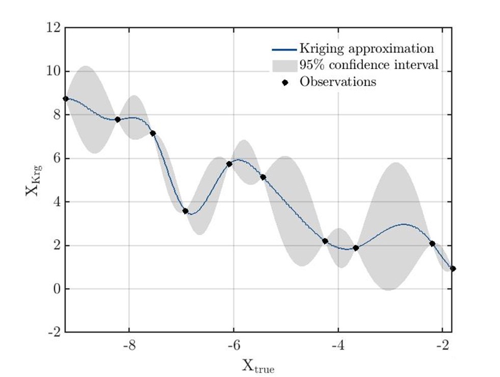
Fig. 36 Example of one-dimensional data interpolation by Kriging with confidence intervals (Image by:T. Albaraghtheh).#
Example#
Here is a simple example of simple Kriging in 1D, this example is created using data mainly consist of 5 observations and mean of the field.
{
import numpy as np
from gstools import Gaussian, krige
# condtions
cond_pos = [0.3, 1.9, 1.1, 3.3, 4.7]
cond_val = [0.47, 0.56, 0.74, 1.47, 1.74]
# resulting grid
gridx = np.linspace(0.0, 15.0, 151)
# spatial random field class
model = Gaussian(dim=1, var=0.5, len_scale=2)
krig = krige.Simple(model, mean=1, cond_pos=cond_pos, cond_val=cond_val)
krig(gridx)
ax = krig.plot()
ax.scatter(cond_pos, cond_val, color="k", zorder=10, label="Conditions")
ax.legend()
}
This code and further examples can be found here https://github.com/GeoStat-Framework
Kriging Toolboxes And Libraries#
Several toolboxes and libraries are developed for Kriging. These toolboxes and libraries are developed in MATLAB, Python, C++ etc. Here is some example of them :
MATLAB (the functioning of these libraries was checked by T. Albaraghtheh)
UQLab (https://www.uqlab.com/kriging-user-manual)
Jiexiang WEN (2023). KrigingToolbox (https://www.mathworks.com/matlabcentral/fileexchange/59960-krigingtoolbox) .
Rafnuss (2023). Area-to-point Kriging (https://github.com/Rafnuss-PhD/A2PK), GitHub
James Ramm (2023). Kriging and Inverse Distance Interpolation using GSTAT (https://www.mathworks.com/matlabcentral/fileexchange/31055-kriging-and-inverse-distance-interpolation-using-gstat).
Mohamed Aissiou (2023). Parametric Kriging (https://www.mathworks.com/matlabcentral/fileexchange/50059-parametric-kriging).
Jiexiang WEN (2023). KrigingToolbox (https://www.mathworks.com/matlabcentral/fileexchange/59960-krigingtoolbox).
jBuist (2023) kriging(x,y,z,range,sill) (https://de.mathworks.com/matlabcentral/fileexchange/57133-kriging-x-y-z-range-sill?s_tid=srchtitle)
Python Detailed review on Python Toolboxes for Kriging Surrogate Modelling is provided by Faraci et al., 2022 [Faraci et al., 2022]
UQ[py]Lab (https://uqpylab.uq-cloud.io/)
scikit-learn
OpenTURNS (General UQ software)
SMT (general library for surrogate models)
OpenTURNS
Case Study#
See Modelling the Degradation of Biodegradable Implants for the application of Kriging to model the complex degradation of biodegradable magnesium-based implants.
References#
- BLGyimothy10
Sandor Bilicz, Marc Lambert, and Sz Gyimóthy. Kriging-based generation of optimal databases as forward and inverse surrogate models. Inverse problems, 26(7):074012, 2010.
- BottcherLF+21
Maria Böttcher, Ferenc Leichsenring, Alexander Fuchs, Wolfgang Graf, and Michael Kaliske. Efficient utilization of surrogate models for uncertainty quantification. PAMM, 20(1):e202000210, 2021.
- CLLZ20(1,2,3)
Kai Cheng, Zhenzhou Lu, Chunyan Ling, and Suting Zhou. Surrogate-assisted global sensitivity analysis: an overview. Structural and Multidisciplinary Optimization, 61:1187–1213, 2020.
- Cla77
Isobel Clark. Practical kriging in three dimensions. Computers & Geosciences, 3(1):173–180, 1977.
- FBG22
missing booktitle in inproceedings
- GHO+17
Roger Ghanem, David Higdon, Houman Owhadi, and others. Handbook of uncertainty quantification. Volume 6. Springer, 2017.
- Kle09(1,2)
Jack PC Kleijnen. Kriging metamodeling in simulation: a review. European journal of operational research, 192(3):707–716, 2009.
- SFK08
András Sobester, Alexander Forrester, and Andy Keane. Engineering design via surrogate modelling: a practical guide. John Wiley & Sons, 2008.
- SMW17(1,2,3)
Bruno Sudret, Stefano Marelli, and Joe Wiart. Surrogate models for uncertainty quantification: an overview. In 2017 11th European conference on antennas and propagation (EUCAP), 793–797. IEEE, 2017.
- WWYC21(1,2)
Kaiwen Wang, Yinan Wang, Xiaowei Yue, and Wenjun Cai. Multiphysics modeling and uncertainty quantification of tribocorrosion in aluminum alloys. Corrosion Science, 178:109095, 2021.
- ZCL11
Liang Zhao, KK Choi, and Ikjin Lee. Metamodeling method using dynamic kriging for design optimization. AIAA journal, 49(9):2034–2046, 2011.
Contributors#
Houda Yaqine, Berit Zeller-Plumhoff