Stochastic Representation of a Reaction Model

Part of a series: Uncertainty Quantification for a Dynamical Model.

Follow reading here

Real world phenomena that are described by reaction systems typically evolve over time stochastically. It is hardly possible to predict the spread of a disease or the variation of gene expression exactly. The dynamics are often subject to randomness induced by internal and external factors [Warne et al., 2019]. In order to capture this behaviour, the dynamics can be characterised by a stochastic process if certain assumptions are satisfied. Within this article, if not stated otherwise, we adopt the notation from the preceding article about reaction systems.

According to [Gillespie, 1992], we impose the assumptions that the system is well-mixed and in thermal equilibrium. It implies that spatial positions of individuals can be ignored and that the dynamics only depend on the current number of each object type. Besides, external parameters, such as temperature, can be neglected. Then, [Gillespie, 1992] shows that the system dynamics follow a Markov jump process (MJP) \(X=(X(t))_{t\ge 0}\), with \(X(t)=(X_1(t),\dots,X_N(t))\). An MJP is a special case of a Markov process that is continuous in time with discrete state space. So, note that \(X=(X(t))_{t\ge 0}\) now defines a stochastic process, i.e. a family of multi-dimensional random variables \(X(t)\) for time points \(t\ge0\). The integer-valued random variable \(X_i(t)\) depicts the random number of individuals of object \(i\) at time point \(t\). In the previous article, the temporal dimension plays a minor role and the state variable \(X\) is considered to be deterministic. Thorough and formal introductions to Markov processes and stochastic processes in general can be found, for example, in [Bass, 2011, Kallenberg, 2021].

Chemical Master Equation

The chemical master equation (CME) is a partial differential equation that describes the time evolution of the state transition distributions of a MJP \(X\). The CME is a special case for MJPs of the more general Chapman-Kolmogorov equation (CKE) for arbitrary Markov processes. Another analogous and popular example of a CKE is the Fokker-Planck equation for diffusion processes [Fuchs, 2013].

Before we are able to formulate the CME, we need to introduce some more notation. Given that \(X(t)=x\), for some fixed \(t\ge0,~x\in\mathbb{N}_0^N\), the probability that reaction \(R_r\) occurs within an infinitesimal time interval \([t,t+dt)\) is denoted by \(a_r(x)dt\), where \(a_r\colon\mathbb{N}_0^N\to\mathbb{R}_+\) is the propensity function of reaction \(R_r\).

This function classically obeys “the law of mass action” that goes back to [Waage et al., 1986] (English translation of the original article from 1864). It states that the probability of reaction \(R_r\) to happen depends on its reaction rate \(c_r\) and the number of combinations of reacting objects. Thus, a common choice of \(a_r\) is [Schnoerr et al., 2017, Wilkinson, 2019]

(2)\[ \begin{align} a_r(x)=c_r\prod_{i=1}^N \binom{x_i}{s_{ir}}=c_r\prod_{i=1}^N\frac{x_i!}{(x_i-s_{ir})!s_{ir}!}. \end{align} \]

Moreover, we denote the probability of the system to be in \(x\in\mathbb{N}_0^N\) at time \(t\ge0\) by \(P(x,t)=P(x,t|x(0),t_0)\) conditioned on the event that it was in state \(x(0)\in\mathbb{N}_0^N\) at time \(t_0\le t\). The change in \(P(x,t)\) over time is described by the CME which states [Gillespie, 1992]

(3)\[ \begin{align} \frac{\partial}{\partial t}P(x,t)=\sum_{r=1}^M \left(a_r(x-v_r)P(x-v_r,t)-a_r(x)P(x,t)\right). \end{align} \]

In plain words, the probability of the system of being in \(x\) at time \(t\) after an infinitesimal time step consists of two parts. The first part \(a_r(x-v_r)P(x-v_r,t)\) on the right-hand side of Equation (3) represents the probabilities of reaching state \(x\) at \(t\) due to a reaction \(r\) after having been in a different state. The second part \(a_r(x)P(x,t)\), however, corresponds to transitions to another state due to a reaction \(r\) and has to be subtracted.

The following example might clarify the meaning of the CME on the basis of the running example from the preceding article.

Example

In the context of this example of a simple reaction system, the propensity functions defined in Equation (2) are given by

\[ \begin{align*} a_1(x)=c_1,\qquad a_2(x)=c_2x_1,\qquad a_3(x)=c_3x_2. \end{align*} \]

Consequently, the CME reads in this case

\[\begin{split} \begin{align*} \frac{\partial}{\partial t}P(x,t)=&\left(c_1P(x-v_1,t)-c_1P(x,t)\right)+\left(c_2(x_1+1)P(x-v_2,t)-c_2x_1P(x,t)\right)\\ &+\left(c_3(x_2+1)P(x-v_3,t)-c_3x_2P(x,t)\right). \end{align*} \end{split}\]

In general, the CME defined in Equation (3) might not admit an analytical solution. In order to study the behaviour of such a system, simulation and approximation methods are commonly used instead.

Simulation

Stochastic simulation methods are able to simulate sample paths of any MJP. The most fundamental algorithm is the stochastic simulation algorithm (SSA). The algorithm was introduced in [Gillespie, 1976, Gillespie, 1977] and it is also known as Gillespie’s algorithm according to its originator. The following formulations are based on [Fuchs, 2013, Wilkinson, 2019].

The exact simulation of any MJP relies on the fact that the waiting time \(\tau\) from a reaction occurring at time \(t>0\) to a next reaction at time \(t+\tau\) is a random variable that is exponentially distributed with rate

\[ \begin{align*} a_0(x(t))=\sum_{r=1}^M a_r(x(t)). \end{align*} \]

The probability of reaction \(R_r\) to happen at \(t+\tau\) is then given by \(\frac{a_r(x(t))}{a_0(x(t))}\). Algorithm 1 depicts the complete iterative procedure of simulated reactions on a time interval \([t_0,T]\) yielding a sample path of a MJP on this interval.

Algorithm 1: Gillespies’s algorithm

Inputs Initial parameters \(t_0>0\) and \(x(0)\in\mathbb{N}_0^N\), final time point \(T>t_0\), propensity functions \(a_r,~r=1,\dots,M\).

Initialization with \(t=t_0\) and \(x(t)=x(0)\).
While \(t<T\)
  Calculate \(a_r(x(t))\), for \(r=1,\dots,M\), and \(a_0(x(t))\).
  Draw \(\tau\sim Exp(a_0(x(t)))\) and set \(\tau^*=\min\{\tau,T-t\}\).
  Draw index \(j\in\{1,\dots,M\}\) with probabilities \(\frac{a_j(x(t))}{a_0(x(t))}\).
  Set \(x(s)=x(t)\) for all \(s\in(t,t+\tau^*)\) and \(x(t+\tau^*)=x(t)+v_j1_{(\tau^*=\tau)}\).
  Set \(t=t+\tau\).
End

Output A sample path \(x(t),~t\in[t_0,T]\), of a MJP \((X_t)_{t\in[0,T]}\).

Gillespie’s algorithm produces a sample path of an underlying MJP. Since it is a probabilistic algorithm, two simulated path of the same system never coincide. In Fig. 22, trajectories from the above expample are depicted. The sample path fully obey the probability distributions of the process that are determined by the CME. Gillespie’s algorithm is therefore referred to as an “exact” [Gillespie, 1992] algorithm. The algorithm is still subject of ongoing research and extensions have been developed. Some important modifications are outlined in [Warne et al., 2019]. All these exact methods usually go along with high computational costs for larger systems that involve numerous reactions that need to be simulated. Approximate algorithms, as the “tau-leaping method” [Gillespie, 2001], are more efficient in that regard.

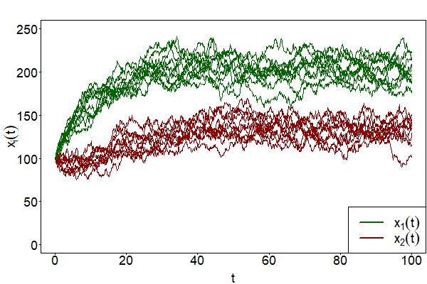
Fig. 22 10 trajetories of the 2-dimensional MJP from the example above generated by Gillespie’s algorithm with \(c_1=20,~c_2=0.1,~c_3=0.15,~x_1(0)=100\) and \(x_2(0)=100\)

The CME admits an analytic solution only in a few special cases [Schnoerr et al., 2017]. Therefore, the likelihood function of an MJP is, in general, not available in order to infer model parameters statistically. This problem can be circumvented by approximations of MJPs or likelihood-free approaches. The former is covered in more detail in the next article in this series.

References

Bas11

Richard F. Bass. Stochastic processes. Volume 33 of Cambridge series in statistical and probabilistic mathematics. Cambridge University Press, Cambridge, 1 edition, 2011.

Fuc13(1,2)

Christiane Fuchs. Inference for Diffusion Processes : With Applications in Life Sciences. Springer, 2013.

Gil76

Daniel T. Gillespie. A general method for numerically simulating the stochastic time evolution of coupled chemical reactions. Journal of Computational Physics, 22:403–434, 1976.

Gil77

Daniel T. Gillespie. Exact stochastic simulation of coupled chemical reactions. The Journal of Physical Chemistry, 81:2340–2361, 1977.

Gil92(1,2,3,4)

Daniel T. Gillespie. A rigorous derivation of the chemical master equation. Physica A, 188:404–425, 1992.

Gil01

Daniel T. Gillespie. Approximate accelerated stochastic simulation of chemically reacting systems. Journal of Chemical Physics, 115:1716–1733, 2001.

Kal21

Olav Kallenberg. Foundations of Modern Probability. Springer, 3 edition, 2021.

SSG17(1,2)

David Schnoerr, Guido Sanguinetti, and Ramon Grima. Approximation and inference methods for stochastic biochemical kinetics - A tutorial review. Journal of Physics A: Mathematical and Theoretical, 50:1–60, 2017.

WGA86

Peter Waage, Cato M. Gulberg, and Henry I. Abrash. Studies concerning affinity. Journal of Chemical Education, 63:1044–1047, 1986.

WBS19(1,2)

David J. Warne, Ruth E. Baker, and Matthew J. Simpson. Simulation and inference algorithms for stochastic biochemical reaction networks: From basic concepts to state-of-the-art. Journal of the Royal Society Interface, 2019.

Wil19(1,2)

Darren J. Wilkinson. Stochastic Modelling for Systems Biology. Chapman & Hall/CRC, 3rd edition, 2019.

Authors

Julian Wäsche

Contributors

Houda Yaqine